Now that you've seen QGIS and OGR in action with vector data, you'll get some experience processing raster data. For this exercise, we're going to start with a 30-meter resolution digital elevation model (DEM) for Philadelphia. I obtained this from the USGS National Map Viewer. We'll use a combination of GDAL tools (some of them wrapped in a nice QGIS GUI) to make a nice-looking terrain background for a basemap. This will be accomplished by adding a DEM, a hillshade, and a shaded slope layer together. I have based these instructions on this tutorial by Mapbox that I encourage you to read later if you would like further detail.
Download the Lesson 3 raster data
Extract the data to a folder named PhiladelphiaElevation, such as c:\data\PhiladelphiaElevation. This will contain a single dataset called dem. In the interest of saving time and minimizing the download size, I have already clipped this dataset to the Philadelphia city boundary and projected it to EPSG:3857 for you. If you need to do this kind of thing in the future, you can use the Raster > Projections > Warp command in QGIS, which invokes the gdalwarp command.
- Launch QGIS and use the Add Raster Layer
 button to add dem to your map.
Don't add any vector layers right now. See the note at the end of this walkthrough if you are eventually interested in overlaying shapefiles with your terrain. - Create a hillshade by selecting dem in the table of contents and clicking Raster > Analysis > Hillshade. Save the hillshade as a TIF file named hillshade, and set the parameters as shown in the image below. Then press Run to execute the command.
Note that if you prefer the command line environment, you can make your future hillshades using the gdaldem hillshade command.
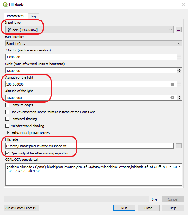 Figure 3.12 Hillshade tool GUI
 - Create a slope surface by highlighting your dem layer in the table of contents and clicking Raster > Analysis > Slope. Save it as a TIF named slope and keep the rest of the defaults. Each pixel in this surface has a value between 0 and 90 indicating the degree of slope in a particular cell.
Now let's shade the slope to provide an extra measure of relief to the hillshade when we combine the two as partially transparent layers. - Create a new text file containing just the following lines, then save it in your PhiladelphiaElevation folder as sloperamp.txt.
0 255 255 255
90 0 0 0
This creates a very simple color ramp that will shade your slope layer in grayscale with values toward 0 being lighter and values toward 90 being darker. When combined with the hillshade, this layer will cause shelfs and cliffs to pop out in your map. - Open your OSGeo4W command line window and use the cd command to change the working directory to your PhiladelphiaElevation folder.
- Run the following command to apply the color ramp to your slope:
gdaldem color-relief slope.tif sloperamp.txt slopeshade.tif
You just ran the gdaldem utility, which does all kinds of things with elevation rasters. In particular, the color-relief command colorizes a raster using the following three parameters (in order): The input raster name, a text file defining the color ramp, and the output file name.
If you add the resulting slopeshade.tif layer to QGIS, you should see this:Now let's switch back to the original DEM and use the same command to put some color into it. Just like in the previous step, you will define a simple color ramp using a text file and use the gdal-dem colorrelief command to apply it to the DEM.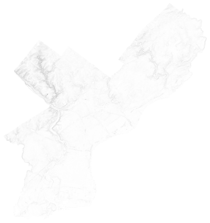 Figure 3.13 Hillshade results
 - Create a new text file and add the following lines (make sure your software doesn't copy it as one big line; there should be line breaks in the same places you see them here). Then save it in your PhiladelphiaElevation folder as demramp.txt.
1 46 154 88
100 251 255 128
1000 224 108 31
2000 200 55 55
3000 215 244 244
Note that the first value in the line is the elevation value of the raster, and the next three values constitute an RGB color definition for cells of that elevation. This particular ramp contains elevations well beyond those seen in Philadelphia, just so you can get an idea of how these ramps are created. I have adjusted the ramp so that lowlands are green and the hilliest areas of Philadelphia are yellow. If we had high mountains in our DEM, brown and other colors would begin to appear. - Run the following command:
gdaldem color-relief dem.tif demramp.txt demcolor.tif
When you add demcolor.tif to QGIS, you should see something like this:This looks good, but the No Data values got classified as green. We need to clip this again. This is a great opportunity for you to practice some raster clipping in QGIS.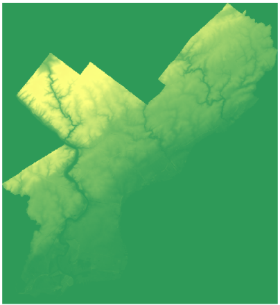 Figure 3.14 DEM sample
 - In QGIS, click Raster > Extraction > Clip raster by mask layer and set up the parameters as below. Make sure you clip demcolor to the city_limits.shp polygon from the previous walkthrough (it should be in PhiladelphiaBaseLayers\clipFeature) and to set the nodata value parameter to 0. Notice that at the bottom of this dialog box, the full gdalwarp syntax (used for clipping) appears in case you ever want to run this action from the command line. This can be a helpful learning tool! Make sure your output file name ends in ".tif" so that the -of GTiff option is added to the gdalwarp command.
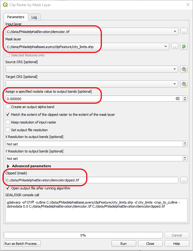 Figure 3.15 Clipper GUI
Now, let's add these together. - Create a new map in QGIS and add the clipped colorized DEM. Then add the hillshade with a 40% opacity. Then add the slopeshade with the 40% opacity. You should get something like below:
Now, play around with the transparencies to suit your liking. You can even re-run the colorization commands to apply different ramps.
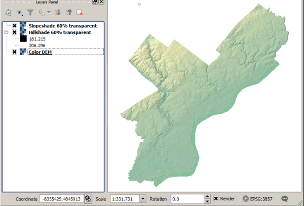 Figure 3.16 Sample map output in QGIS
This type of terrain layer, when overlayed by a few other vector layers, could act as a suitable basemap layer in a web map. In a future lesson, you'll learn how you could create tiles of this type of layer to bring into your web map.
Saving the data for future use
Just like in the previous walkthrough, you will copy your final datasets into your main Philadelphia data folder for future use.
Use Windows Explorer or an equivalent program to copy hillshade.tif, slopeshade.tif, and demcolorclipped.tif into the Philadelphia folder (such as c:\data\Philadelphia) that you created in the previous walkthrough.