Identifying Patterns - Chaotic Periodicity

Read...

In the atmosphere and ocean, there are some common climatic patterns. A lot of these climatic patterns result in teleconnections - meaning when certain phases of this pattern occur, we can expect a particular meteorological feature elsewhere (spatially). Teleconnections are very useful for forecasting! You should note that the goal right now is simply for you to identify patterns in a dataset, know which variables you need to detect those patterns, and the potential teleconnections. In future lessons, you will have to account for these patterns when performing certain time series analyses. So being able to identify these patterns is key! If you are interested, there is a pretty good blog by NOAA climate that includes articles on natural climate patterns.

Teleconnections

Before we go into specifics, let’s talk a little bit more about teleconnections. The reason we are interested in these slowly varying multi-region patterns is that if we are in certain phases of these patterns, we can sometimes infer something about the weather (i.e., temperature, precipitation, etc.). This is a result of teleconnections.

Teleconnections are defined in the AMS (American Meteorological Society) glossary as a “linkage between weather changes occurring in widely separated regions of the globe.” Something occurring in one geographic location can impact another location. These teleconnections can help identify certain scenarios that may play out. For example, if we know increased SST in one region can bring droughts in another location, we can expect/predict when those droughts may occur based on observing the SST.

There are many atmospheric/oceanic teleconnections (ENSO, AO, NAO, MJO). These teleconnections are generally referred to as long timescale variability, but they can last for several weeks to several months and even years. Because of their long timescale, these teleconnections can aid in the understanding of both the inter-annual variability and inter-decadal variability. For more information on the general concept of teleconnections in weather and climate, check out this CPC site.

Now, let’s start looking at some common chaotic patterns that you may find in this field. 

ENSO

Out of all the patterns that exist in the atmosphere and or ocean, ENSO is probably the most well known. You’ve probably heard about it being talked about during extreme floods or droughts. The El Niño-Southern Oscillation (ENSO) is a natural pattern characterized by the fluctuations of Sea Surface Temperatures (SST) in the equatorial Pacific.

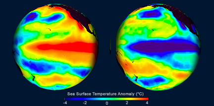
With respect to ENSO, there are two main phases: warmer than normal central and eastern equatorial Pacific SSTs (called El Niño) and cooler than normal SSTs in central and eastern Pacific (called La Niña). Below is an example of El Niño conditions on the left and La Niña on the right.

You can check out the current conditions here. These states last about 9-12 months, peaking in December-April and decaying during the months of May to June. Prolonged episodes have lasted 2 years in the past. The periodicity is chaotic but, on average, we expect the pattern to reoccur every 3-5 years.

There are several ways to monitor the ENSO state. One is using the Oceanic Niño Index (ONI). You can read more about the index here. In short, a 3-month running SST anomaly mean is measured in an area called the Niño 3.4 region. If the value is above 0.5°C, then it is considered to be in the warmer phase; if it’s less than -0.5°C, it is characterized as being in the cooler phase. To be defined as the La Niña or El Niño phase, there must be 5 consecutive months in which the 3-month running average was below or above the threshold.

So why do we care about an anomaly in the equatorial Pacific Ocean? Well, it has to do with the teleconnections. The impacts of an El Niño or a La Niña vary by not only region but when, temporally, the phase is occurring.

For El Niño, this plot below shows the teleconnections during the months of December through February on the left and June through August on the right.

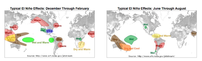
This figure shows the general impact. For example, the southwestern US generally has wetter than normal conditions during the months of December - February when an El Niño event is occurring.

Similarly, we expect teleconnections for La Niña. During the months of December through February, the typical La Niña effects are displayed on the left, while the months of June through August are displayed on the right.

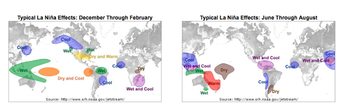
Again, we discuss the general regions as being wetter or drier than normal, and cooler or warmer than normal. For example, during the months of June through August, the western coast of South America extending from Peru down into Chile is generally characterized by cooler than normal conditions when the La Niña phase occurs.

To summarize:

1. ENSO is characterized by fluctuations in SST.
2. We use the Oceanic Niño Index to determine the phase.
   1. If there are 5 consecutive months with an anomaly greater than 0.5°C, then we are in the warm phase called El Niño.
   2. If there are 5 consecutive months with an anomaly less than -0.5°C, then we are in the cool phase called La Niña.
3. The general periodicity is 3-5 years.
4. Impacts vary not only by region but by the month the phase is occurring in.

AO and NAO

The Arctic Oscillation (AO) and the North Atlantic Oscillation (NAO) are characterized by changes in pressure or geopotential heights.

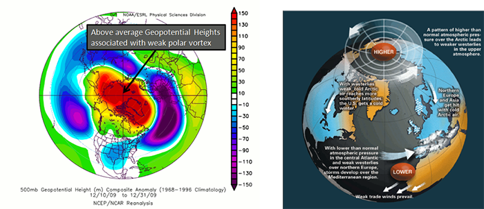
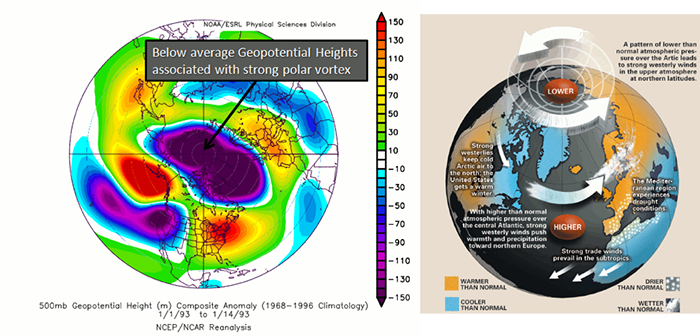
The AO consists of a negative and positive phase. If we know the phase of the AO, we have some clues about the large-scale weather patterns a week or two in the future. The negative phases occur when above-average geopotential heights are observed in the Arctic. This means there is a weaker than normal polar vortex. During this phase, the westerlies weaken, resulting in cold air plunging into the middle of the US and Western Europe. The figure on the left shows the above average geopotential heights associated with a weak polar vortex, highlighting the negative AO phase, while the right figure shows the consequences of this pattern change.

In contrast, the positive phase occurs when geopotential heights are below average in the Arctic. This means there is a stronger than normal polar vortex. During this phase, the westerlies are stronger, resulting in milder weather in the US and weaker storms. The figure on the left shows the below average heights associated with a strong vortex, highlighting the positive AO phase. The figure on the right shows the impacts of this pattern.

To check out the current state of the AO, look at this site. The AO index is computed by projecting the daily (00z) 1000 mb height anomalies poleward of 20°N onto the pattern of the AO. If the AO index is positive, it is in the positive phase, and if it’s negative, it’s in the negative phase. The AO is important for the weather in North America, but there is no preferred timescale.

To summarize:

1. AO is characterized by changes in geopotential height or pressure in the Arctic.
2. We use the AO index to determine the phase.
   1. If AO index > 0 positive phase.
   2. If AO index < 0 negative phase.
3. There is no general periodicity.
4. The negative phase results in stormy weather in Europe and generally colder weather in the US. During the positive phase, we expect milder weather in the US with droughts in Europe.

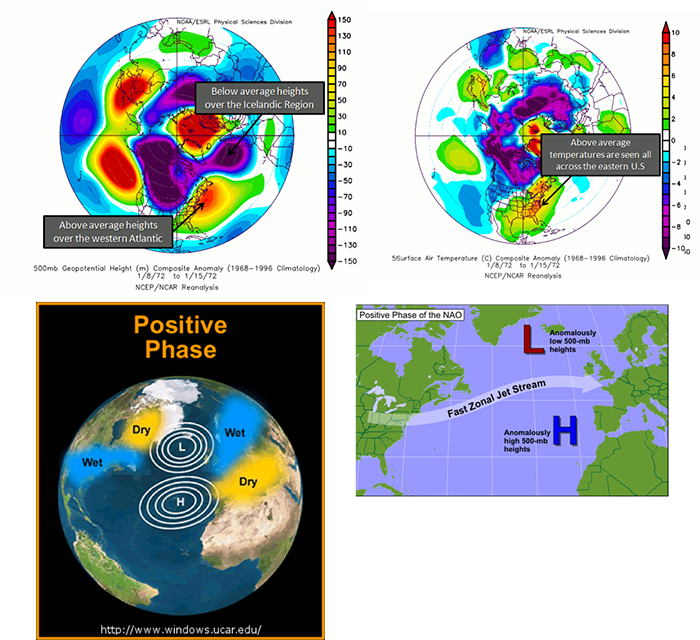
The NAO is similar to the AO, but the geopotential heights are observed near Iceland and the Azores islands in the Atlantic Ocean instead of the Arctic. During a positive NAO, the 500 mb heights over Iceland are anomalously low while the 500 mb heights over the Azores are anomalously high, favoring strong westerlies. During this phase, the temperatures in the eastern US tend to be milder with weaker storms. Northern Europe is also milder, but wetter than average, while central and Southern Europe are drier. The figures below characterize the heights during a positive NAO, the temperature anomalies, and the precipitation anomalies.

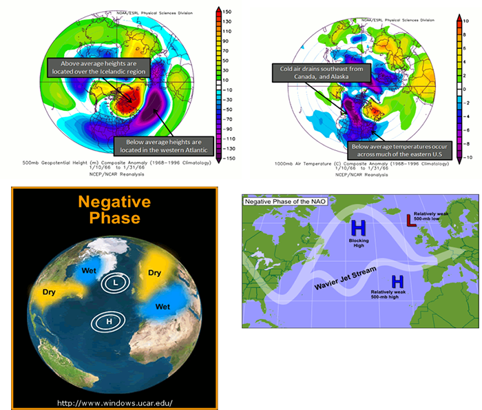
During a negative NAO, the Icelandic height anomalies are high, while the Azores are low. This tends to weaken the westerlies. What results is a pressure high over the North Atlantic that blocks and slows down the progression of a weather system across the US. This favors colder outbreaks in the eastern US and favors the development of strong mid-latitude cyclones leading to East Coast snowstorms. Particularly, during the winter season, a predominantly negative phase can lead to cold snow across the eastern part of the US and Europe. Below are figures demonstrating the cause and impacts of a negative phase.

To see the current NAO state, you can use the NAO index here. A positive NAO index suggests a positive phase, while a negative index suggests a negative phase. Similar to the AO, there is no general periodicity.

To summarize

1. NAO is characterized by changes in geopotential height or pressure near Iceland and the Azores.
2. We use NAO index to determine the phase,
   1. If NAO index > 0 positive phase.
   2. If NAO index < 0 negative phase.
3. There is no general periodicity.
4. The negative phase results in cold, snowy weather across the eastern US and Europe. During the positive phase, milder weather is observed in the eastern US, while wetter than average weather can occur in Northern Europe and drier than average in central and Southern Europe.

You can see that the AO and NAO are very similar, and you might be wondering which one you should use. Some researchers believe the NAO is part of the AO and, therefore, you should use the AO, while others believe the measurements for the NAO are physically more meaningful and, therefore, more representative of the true nature of the westerlies, leading to stronger predictions. You will generally see both oscillations utilized.

PNA

The Pacific-North American (PNA) pattern is a complement to the NAO and is characterized by geopotential heights. It can be used to estimate the state of the westerlies over the Pacific and North America. Research suggests that there is a linkage between the PNA and ENSO.

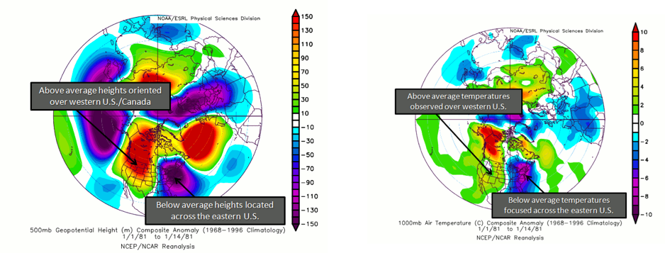
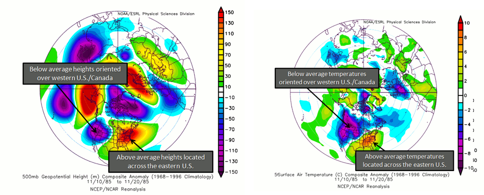
Again, there are two phases. The positive phase consists of above normal geopotential heights over the western US and anomalous lows over the eastern US. During this phase, cold air in Canada is forced southeastward, leading to anomalously low temperatures over the eastern US and anomalously high temperatures over the western US. Cyclogenesis (formation of cyclones) is also enhanced near the west coast of North America. In addition, anomalously high precipitation along the west coast of Canada and the Pacific Northwest is generally observed. A positive PNA tends to dominate during El Niño years. Below is a figure showing the typical geopotential heights during the positive phase and the corresponding temperatures.

During the negative phase, there are anomalously low geopotential heights over the western US with above normal over the eastern US. During this phase, the average temperatures for the western US are low, while for the eastern US they are high. It is more likely that Pacific air can cross the US, limiting outbreaks of cold weather and the development of major cyclones. Precipitation tends to be high in the Mississippi and Ohio Valleys, while the southeastern US is drier. Please note that the precipitation anomalies are less robust when it comes to the PNA than in other patterns. Generally, a negative PNA occurs during La Niña years. Below is a figure showing the typical geopotential heights during the negative phase with the corresponding temperature information.

You can check out the current conditions here using the PNA index. The periodicity is again somewhat spontaneous, but due to the linkage with ENSO, you could expect every 3-5 years.

To summarize:

1. PNA is characterized by changes in geopotential height over the western US and the eastern US.
2. We use the PNA index to determine the phase.
   1. If PNA index > 0 positive phase.
   2. If PNA index < 0 negative phase.
3. There is no general periodicity, but the connection to ENSO might suggest 3-5 years as a starting base.
4. The negative phase brings anomalously low temperatures to the western US and high temperatures to the Eastern US while limiting the outbreak of cold weather and the development of major cyclones. The positive phase forces cold air from Canada over the eastern US with higher than normal temperatures over the western US. Cyclogenesis is also enhanced during this phase.

PDO

The variable of interest for the Pacific Decadal Oscillation (PDO) is SST. The PDO is considered a pattern of Pacific climate variability similar to ENSO. There is a warm and cool phase that can impact hurricane activity, droughts, and flooding. The interaction with ENSO can magnify or weaken the impacts, depending on if they are in phase. Please note that the PDO is still a highly researched teleconnection and not as much is known compared to other patterns. This is partly due to the long periodicity of 20-30 years.

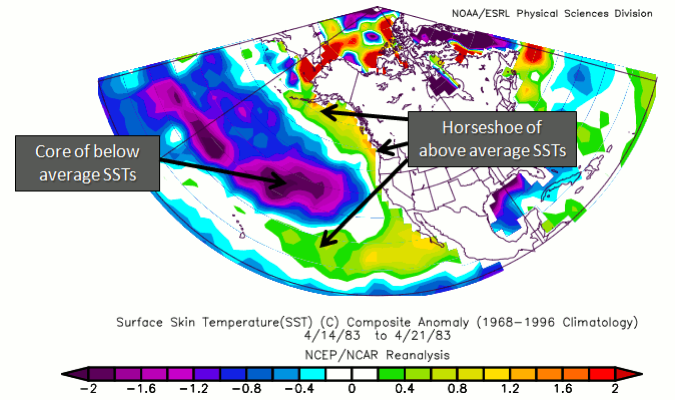
A warm phase of the PDO is characterized by anomalously high SSTs off the coast of North America from Alaska to the equator wrapping around cooler than normal SSTs in a horseshoe-like feature. If a warm PDO coincides with a La Niña, the impacts of a warm PDO weaken. If a warm PDO coincides with El Niño, the impacts magnify. It is believed that a warm PDO can enhance coastal biological productivity in Alaska but inhibit it off the west coast of the US. A warm PDO can result in warmer than average temperatures in the Pacific Northwest, British Columbia, and Alaska, with lower than average temperatures in Mexico and the southeastern US. In terms of precipitation, a warm PDO is associated with above-average precipitation in Alaska, Mexico, and the southwestern US with below average in Canada. Here is an example of the signature SST for a warm PDO.

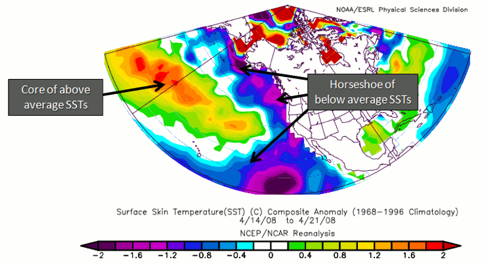
In contrast, the cold phase is the exact opposite in terms of SST, with anomalously low SSTs off the coast of North America wrapping around warmer than normal ones. If a cold PDO coincides with a La Niña, the impacts are magnified. Impacts are exactly opposite than in the warm phase. That is, coastal biological productivity in Alaska is reduced but enhanced off the west coast of the CONUS. Cooler than average temperatures in the Pacific Northwest, British Columbia, and Alaska are observed with higher than average in Mexico and the southwestern US. For precipitation, lower than average is expected in Alaska, Mexico, and the southwestern US, with higher than average in Canada. Here is an example of the signature SST for a cold PDO.

To summarize:

1. PDO is characterized by a horseshoe signature of cold or warm temperatures off the west coast of the US.
2. If the temperatures along the coast are warm (cold), then the PDO is in a warm (cold) phase. If El Niño (La Niña) coincides with the warm (cold) phase, impacts are enhanced.
3. This is a less studied pattern, but the periodicity is believed to be 20-30 years.
4. The warm phases enhance coastal biological productivity in Alaska, while inhibiting it off the west coast of CONUS. During the warm phase, the PDO results in warmer than average temperatures in the Pacific Northwest, British Columbia, and Alaska, with lower than average in Mexico and the southwestern US. A cold phase results in below average precipitation in Alaska and above average in Canada.

MJO

The Madden Julian Oscillation (MJO) is formally an intra-seasonal wave that occurs in the tropics, which manifests itself in the form of alternating areas of enhanced and suppressed rainfall that migrates eastward from the Indian Ocean to the central Pacific Ocean and sometimes beyond. Precipitation will be the variable of interest.

There are 8 phases of the MJO (Wheeler and Hendon 2004), with a timescale of about 6 days for each phase. However, there is large variability in the speed of the progression. A complete cycle can take 30-60 days, but there have been instances near 90 days. In addition, the intensity can be highly variable. Here is an animation of the cycle:

In the video above, blue shades are anomalously high rainfall rates (at least 1 mm/day more than normal), while orange represents low rainfall (at least 1 mm/day less than normal). Note the eastward progression of the MJO as it works through the eight phases (upper right corner of animation).

There are many teleconnections with the MJO. For Tropical connections, the MJO acts as a modulator of global tropical cyclone activity. For Mid-Latitude connections, when the MJO is more intense, a 40% increase in extreme rainfall occurs globally (as compared to a weak MJO). Wintertime floods in the northwest are common when the MJO is in phase 2 or 3, while severe flooding in the northwest is most common in phase 6.

I suggest checking out this summary of the MJO for more detail, as the scope of the pattern is too large to cover everything right here.

To summarize:

1. MJO is characterized by precipitation anomalies that migrate eastward from the Indian Ocean to the central Pacific Ocean.
2. There are 8 phases of the MJO typically lasting 6 days each.
3. The progression is generally 30-60 days long, although a 90-day period has been observed.
4. When the MJO is in phase 2 or 3, flooding during wintertime can occur in the northwest US, while severe flooding occurs during phase 6.