Basics of Time Series Modeling

Read...

Now that we have prepared our data and checked for any missing values, outliers, and inhomogeneity, we can begin talking about modeling. The common goal of a time series analysis is modeling for prediction but, before we dive in, we need to cover the basics. In this section, we will focus on the assumptions required to perform an analysis and how we can transform the data to meet those requirements.

Stationary

The easiest time series to model is one that is stationary. Stationarity is a requirement to perform many time series analyses. Although there are functions in R that will avoid this requirement, it’s important to understand what stationarity means, so you can properly employ these functions. So read on!

There are three criteria for a time series to be considered stationary.

1. The mean of the time series should be constant. It should NOT BE a function of time. Look at the graphs below. Notice the time-dependence increase in the orange one - in that case, the mean value changes with time and would not be considered stationary.
   

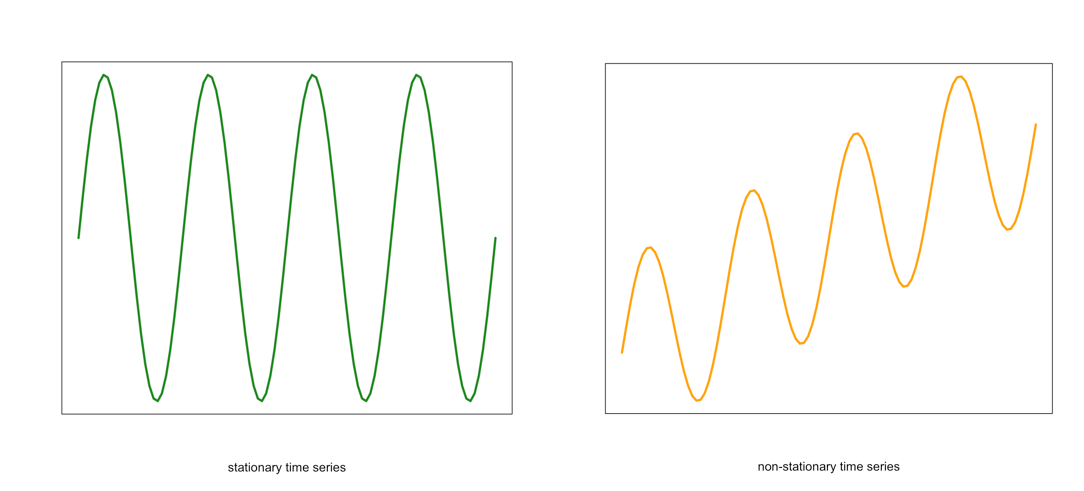   Visual of a stationary (left) and non-stationary (right) time series

   Credit: J. Roman
2. Similarly, the variance should be constant in time. This is called homoscedasticity. Look at the graphs below. Notice how the spread (range in values) changes with time in the orange one. This is an example of a time series that would not be considered stationary by breaking the requirements of homoscedasticity.
   

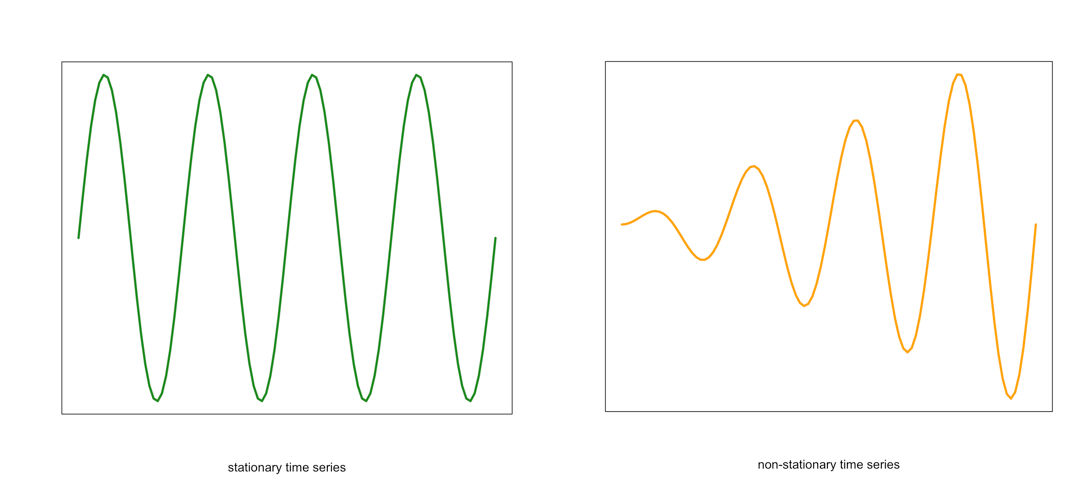   Example of a stationary (left) and non-stationary heteroskedastic (right) time series 

   Credit: J. Roman
3. The last requirement is that the covariance between sequential data points should NOT BE a function of time. Again, look at the graph below. Notice the change in the spread in the time direction of the orange one. This is an example of a time series that is non-stationary and does not meet the requirement of steady covariance.
   

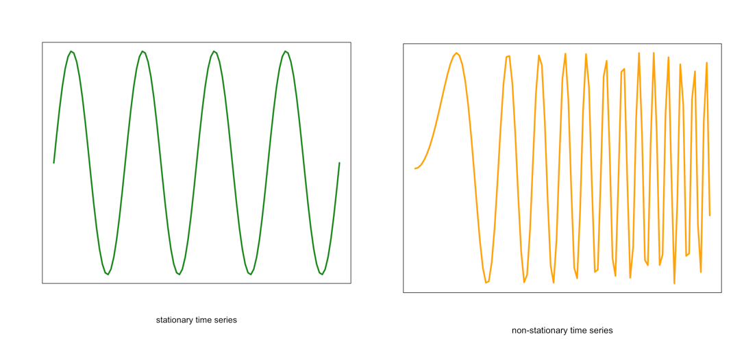   Example of a stationary (left) and non-stationary non-constant covariance (right) time series 

   Credit: J. Roman

If your data meets these assumptions, you are good to go. If not, you need to explore methods for dealing with non-stationary datasets. Continue on to find out what we can do.

Non-stationary

For the purpose of this course, any time series that does not meet the stationary requirements will be called non-stationary. Like I said previously, some functions in R can automatically deal with a non-stationary time series, but there are ways to transform the data to make it stationary.

Data transformations were discussed briefly in Meteo 810. Because of this, I will only provide a review of the more common techniques. I suggest you re-read those sections if you need more of a refresher.

The first data transformation is differencing. Differencing is simply taking the difference between consecutive observations. Differencing usually helps stabilize the mean of a time series by removing the changes in the level of a time series. This, in turn, eliminates the trend. In R, you can use the function ‘diff()’.

We can also compute an anomaly to remove the seasonality cycle or cycles that repeat periodically. To compute the anomaly, we subtract off a climatology (a mean over a pre-determined period). For example, let’s say I have monthly temperature data. We know that the temperature in the Northern Hemisphere is warmest during summer months (JJA) and is coldest in winter (DJF). This is a cycle that repeats every year. We can remove this cycle by subtracting off the monthly climatology. That is subtracting off a mean monthly value. So for a given observation in January, we subtract off the mean of all Januarys in that dataset (or over a predetermined time period). For a February observation, we subtract off the mean of all Februarys, and so on. We are left with an anomaly that has removed this cycle.

The next common method is log. To transform the data this way, we take the natural log of each value. A log transformation is usually used if the variation increases with the magnitude of the local mean (e.g., if the range of potential instrument error increases as the true value increases). In such cases, the log transformation stabilizes the variance. In R, you can use the function ‘log’.

The last transformation we will review is the inverse. The inverse is just the reciprocal of the value (1/x). This is considered a power transformation, similar to the log, and is used to stabilize the variance in situations where small measurements are more accurate than large. In R, you can use the ‘1/x’ command.

When you run into a non-stationary dataset, my recommendation is to attempt a transformation to try and meet the stationary requirement. If this does not work, then you can exploit the functions in R that do not require a stationary dataset.

How to test for stationarity

We’ve discussed the requirements for a time series to be stationary, and I have shown a few figures that display a typical stationary and non-stationary time series. But sometimes it will be very difficult to simply look at the time series and determine if the assumptions are met. So we will talk about different ways to check for stationarity. 

1. Check the ACF and PACF
   The function ‘acf’ estimates the autocorrelation. Autocorrelation is the correlation between elements in time. The correlation coefficient is computed between the values at two different time periods. For example, the value at time t is compared to the value at time t+1, t+2, t+3…. And so on. These are called ‘lags’. Similar to correlation, if the coefficient is close to $\pm$ 1, then the two values are strongly related. Autocorrelation will be discussed in more detail later on. For now, just know that if there is a high autocorrelation (close to $\pm$ 1) for all lags, the time series is not stationary.
   
   The function ‘pacf’ computes the partial autocorrelation. It is similar to the autocorrelation function but controls for the values of a time series at all shorter lags. For example, if you are looking at the correlation between time t and t+3, the partial autocorrelation takes into account the values at time t, t+1, t+2, and t+3. Whereas the autocorrelation only examines the values at time t and t+3. Again, if the correlation is high for all lags, the series is not stationary.
   
   Let’s test this out with our SST data. We will first compute the mean global SST anomaly. To do this, use the code below:
   Show me the code...

   Your script should look something like this:

   # compute global mean
   meanGlobalSSTAnom <- apply(NOAAglobalSSTAnomImpute,3,mean)
   

   Now we can compute the ACF and PACF. Run the code below: 
   You should get the following figures:
   

   ACF (left) and PACF (right) of NOAA global mean SST and air temperature anomalies

   Credit: J. Roman
   The ACF shows strong correlation for all lags, while the PACF does not. So while the ACF suggest non-stationary, the PACF does not. How do we decide what to do? Let’s continue on to find out some more quantitative ways to check for stationarity.
2. Kwiatkowski-Phillips-Schmidt-Shin (KPSS) test
   To confirm your visual results, you can run a KPSS test. The KPSS is a hypothesis test that evaluates whether the data follows a straight line trend with stationary errors. The null hypothesis is that the trend does. The alternative is that it doesn't. So if the p-value is small, we reject the null in favor of the alternative and the trend is assumed to have non-stationary errors.
   
   Let’s test this out with our SST data. Use the code below to compute the KPSS Test
   Show me the code...

   Your script should look something like this:

   # load in tseries library
   library("tseries")
   
   # compute KPSS test 
   kpss.test(meanGlobalSSTAnom, null=”Trend”)
   

   The result is a p-value less than 0.01. This means we reject the null in favor of the alternative. The trend does not have stationary errors, so our time series is not stationary. 
3. Augmented Dickey-Fuller (ADF) test
   Another test is the Augmented Dickey-Fuller t-statistic test. This hypothesis test determines whether the unit root is in a time series. A unit root is a feature in some data that can cause problems in our analysis and suggests that the variable is non-stationary. For this test, the null hypothesis is that the unit root exists in the data. The alternative hypothesis is that it doesn’t exist, and the data is considered stationary. So, if the p-value is small, we reject the null in favor of the alternative suggesting the data is stationary.
   
   Let’s test this out with our SST data. Use the code below to perform this test.
   Show me the code...

   Your script should look something like this:

   # compute ADF test 
   library(tseries) 
   adf.test(meanGlobalSSTAnom)

   The result is a p-value less than 0.01 suggesting the data is stationary. 

There are many more tests out there that you can try. These were just a few examples of what you can do to visualize and quantify the stationary aspect of your dataset. And like the example highlights, you might get conflicting answers. You will have to decide what route is the best route to go based on your results. 

Now test yourself. Using the app below, select a variable from the list and examine the plots and output from the hypothesis tests. Try and decide, based on the quantitative and qualitative results, if the time series is stationary.