Flow Duration Curve

Flow Duration Curve

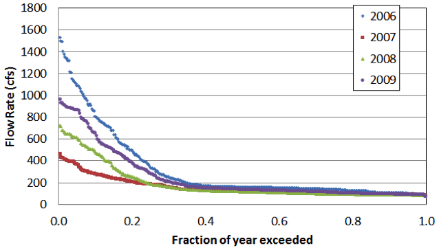
While it can be very informative to study hydrographs and the other flow metrics described above, often an important question often asked about rivers is ‘what percentage of time does flow exceed (or not exceed) a given value (e.g., 100 cfs)?’ It might be important to answer that question to determine the percentage of time when the flow is too low to support a particular fish species. Or it may be important to know what percentage of time the river exceeds a certain value known to cause flood damage. The proportion of time any given flow is exceeded can be determined by generating a flow duration curve. Figure 21 shows the flow duration curve for the hydrograph shown in Figure 21 (2006 water year) as well as the three subsequent years. You can immediately see that the mid and lower flows (exceeded about 40% (or 0.4) of the year) are relatively similar in each year, but the larger flows exhibit quite a bit of variability. In 2007 the highest flow of the year was only a bit over 400 cfs, while it was over 1500 cfs in 2006. The flow that was exceeded 20% of the time (0.2 on the x-axis) was approximately 450 cfs in 2005, but only 200 cfs in 2007.

Figure 22. Flow duration curves for the Logan River, in northern Utah for four different years. As the Logan River is a snow-melt dominated system, observed differences in high flows each year (left side of plot) correlate to differences in snowpack in each of the years.

Source: Patrick Belmont

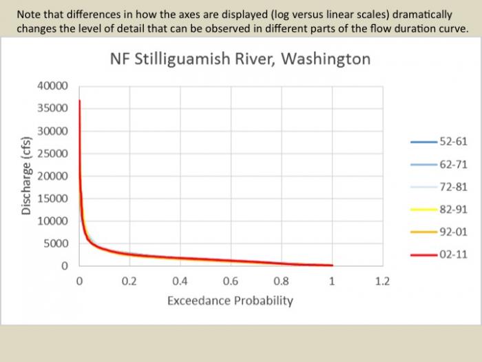
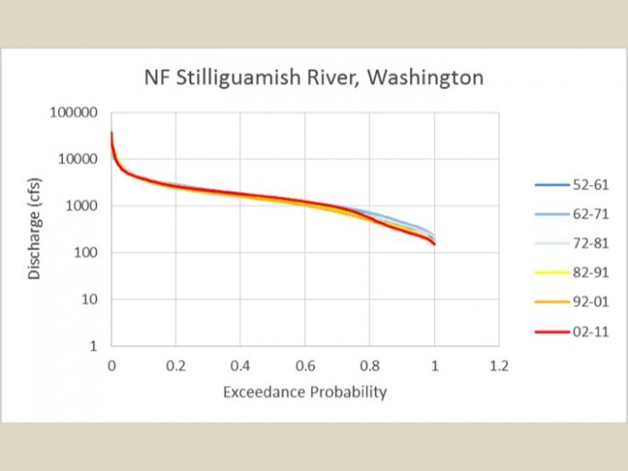
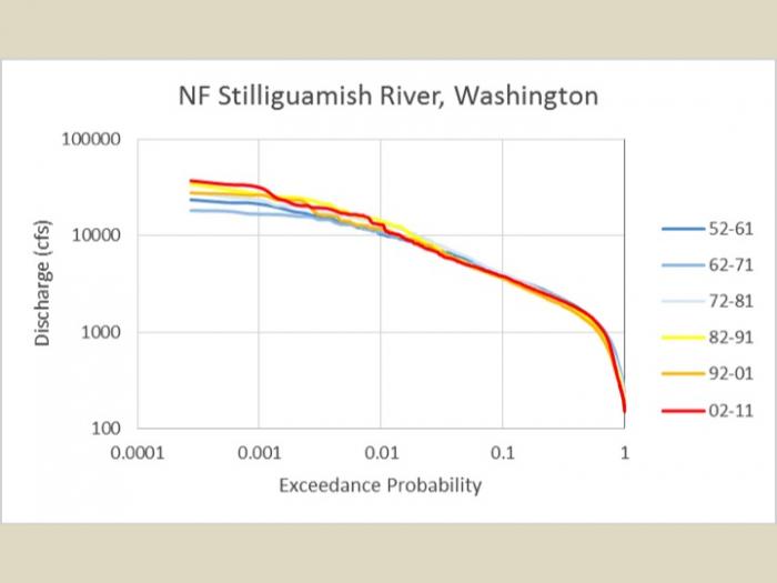
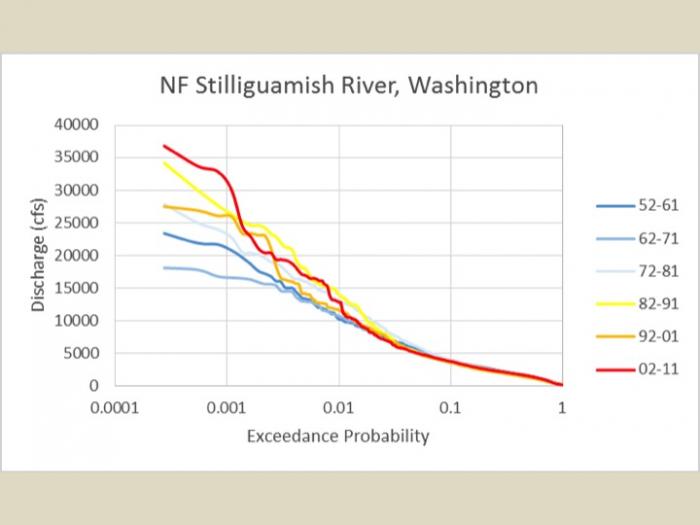
Note that this plot provides detailed information on different parts of the flow duration curve depending on whether you use linear or log scales for the x or y axes (see example from the Stilliguamish River, Washington below in Figures 22-25).

Figure 23. Stilliguamish River, Washington

Source: USGS

Figure 24. Stilliguamish River, Washington

Source: USGS

Figure 25.Stilliguamish River, Washington

Source: USGS

Figure 26. Stillaguamish River, Washington

Source: USGS

Figure 27. Root River, Minnesota

Source: USGS

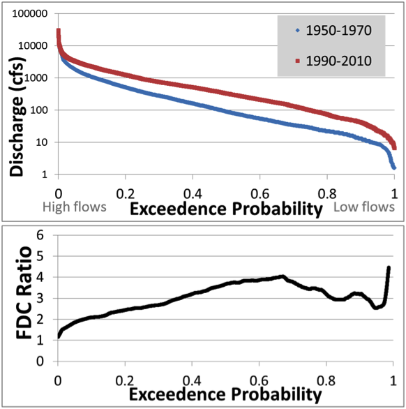
Flow duration curves can be made for a given river over two different time periods to illustrate if/how the range of flows has changed over time. For example, Figure 27 shows flow duration curves for the Le Sueur River in southern Minnesota for two different time periods (1950-1970 in blue, 1990-2010 in red). Note that in these plots the fraction of year exceeded is labeled as ‘exceedance probability’. These two terms are interchangeable, both being computed as:

$$Ep=\frac{R}{\left(n+1\right)}$$

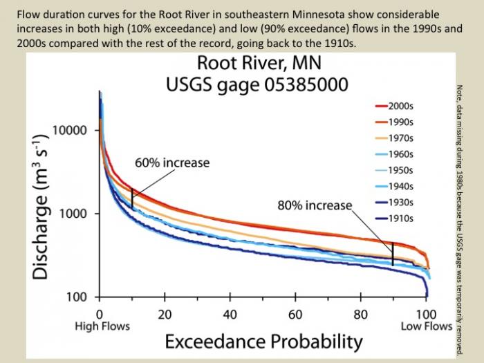
Where E_p is the exceedance probability or the fraction of the year that a given flow is exceeded, R is the rank, and n is the total number of values (365 if you are using daily-averaged flow values for a non-leap year). High flows (toward the left side of each plot) and low flows (toward the right side of each plot) appear not to have changed in the Elk and Whetstone rivers. In the Blue Earth River, low flows (exceeded more than 85% of the time) have not changed much, but mid-range and high flows all appear to have increased. In the Le Sueur River, the full range of flows appears to have increased. Note that the y-axis is plotted on a log scale, so even the modest difference between the two curves represents a significant increase in high flows (e.g., those that are only exceeded 5-10% of the time). The Root River, in southeastern Minnesota, has experienced significant increases in high and low flows within the past two decades, see example above.

Figure 28. Flow duration curves are shown for two different time periods in the Le Sueur River, southern Minnesota. Changes in flows are attributed to changes in artificial drainage of agricultural fields, as well as changes in precipitation and crop type. See Schottler et al., (2014) Hydrological Processes for more information.

Source: Patrick Belmont