1.7 Growth, Delays, and Tipping Points

1.7 Growth, Delays, and Tipping Points

Growth

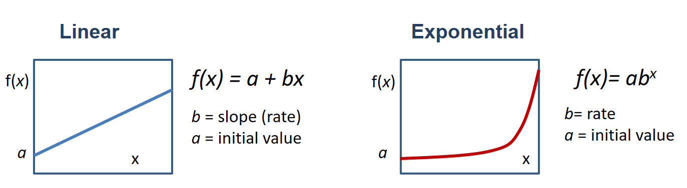
Since this lesson has some analysis and discussions of growth, it would be interesting to see how growth happens in system dynamics. Two types of growth we want to pay attention to are linear and exponential. Linear growth is when a value grows at a constant rate (slope). Positive couplings in systems are a usual cause of linear growth. For example, more product sold means higher profit; more fuel burned, more energy is released – those are simple observations. Exponential growth is different – it goes at an increasing rate – it accelerates! Systems with positive feedback loops often exhibit exponential growth, because the initial stock is continuously compounded by the positive couplings included in the loop.

Mathematically, these two types are schematically represented in Figure 1.22.

Figure 1.22. Graphic and mathematical representation of linear (left) and exponential (right) growth.

Credit: Mark Fedkin

One of the examples shown in the previous section was about the bank account with interest. Adding interest to your balance increases the initial stock and thus earns you higher interest. This illustrates how a positive feedback works. Another example is population growth. When unhindered, the positive feedback loops are expected to cause exponential changes in system stocks.

Example: How to Use Exponential Formula

f(x) = ab^x

This mathematical expression generically represents an exponential process. In this formula:

f(x) is a function – the amount we try to track over time. In the case of a bank account, it will be the account balance, or in case of population growth - the number of chickens, bacteria, or people.

a is the initial value, e.g., the account balance to start from or starting population of species.

b is the base, which indicates the factor by which the initial amount changes per unit of time. For example, if the number of bacteria doubles every hour, b=2. Or if the bank account grows by 6% every year, b=1.06.

x is an exponent, which acts essentially as a time coordinate. For example, if you try to calculate the function for 10 hours ahead, x=10.

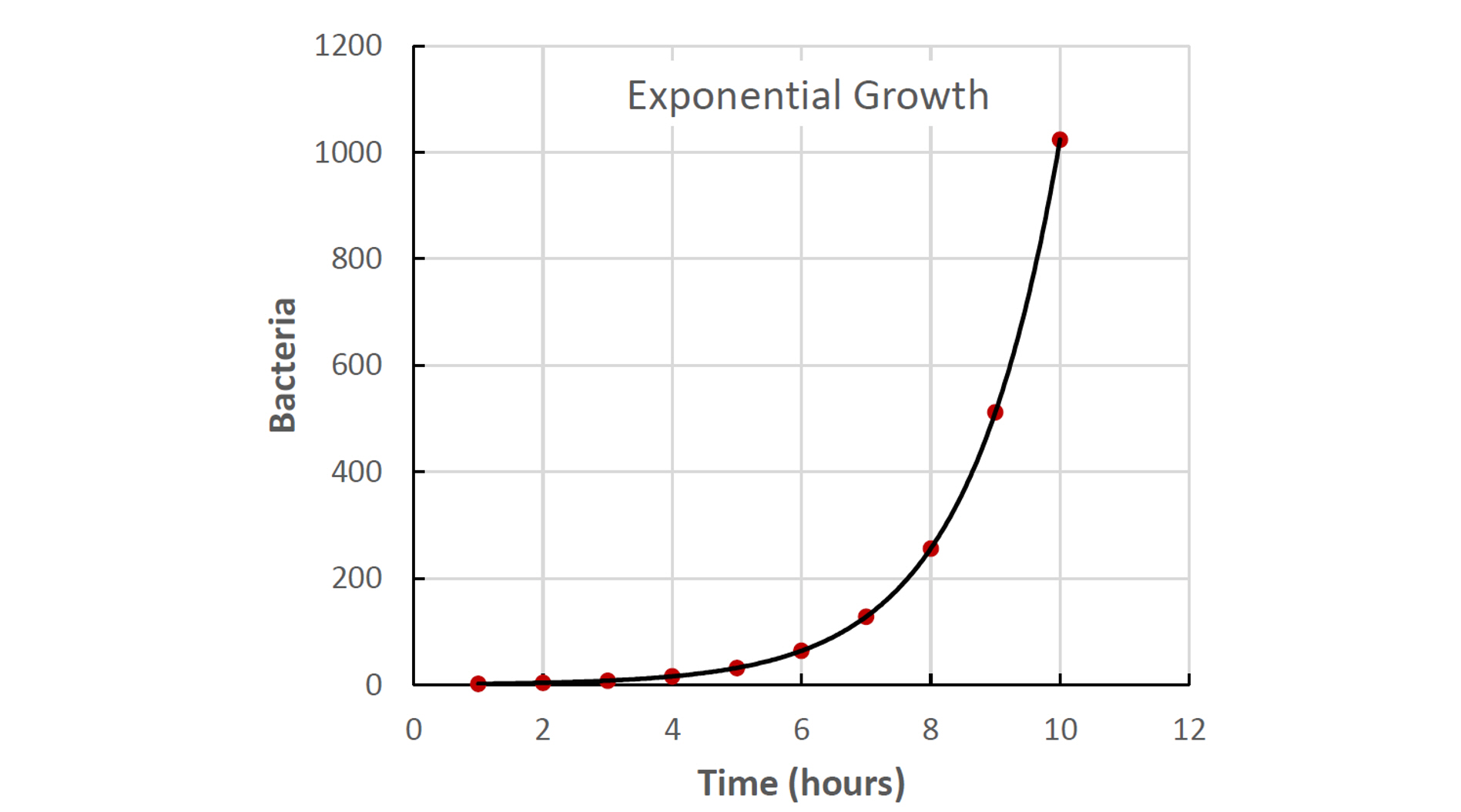
Starting with 1 bacteria (a=1) and hourly doubling increase (b=2), in 10 hours we will have f(x) = 1 x 2¹⁰ = 1024 bacteria.

Figure 1.23. Exponential growth with doubling rate.

Credit: Mark Fedkin

From the above examples, we can make a few interesting observations:

• Exponential growth starts slow, but it becomes fast very fast.
• The result of exponential growth is very hard to predict intuitively because we are used to thinking linearly
• Very often, exponential growth is the result of positive feedback in the system
• Negative (balancing) feedbacks are one way to limit system growth
• Exponential growth cannot be sustainable within a finite-size system and reaching capacity crisis is only a matter of time.

Delays

When we discussed couplings in systems, we mentioned that such causal connections exist when A affects B in either a positive or negative way, but we did not pay much attention to how fast that happens. Some changes can be almost instantaneous (or at least seem like that). For example, clouds moving across the sky immediately change the flow of solar energy coming down to earth, and suddenly we feel cooler, or if the sunlight is used for electric generation, the voltage of the solar panel quickly drops. But other changes may take minutes, hours, days, years, and even millennia. That essentially means we have a delay between the cause and its effect.

Examples of systemic delays are multiple. Here are just a few:

• Incubational period of a viral disease – time between virus entering the body and symptoms
• Forest growth – time between seeds germinate in the soil and trees reaching a certain height;
• Greenhouse effect in climate – time between atmospheric carbon dioxide concentration increase and global temperature increase
• Prices in the market – time between supply or demand grow and decision to adjust the price for a product.

The larger the system, the greater the volume of the stock, the longer it takes for it to respond to change. That is why planetary system often experiences changes (climate, ocean chemistry, geochemical cycles) with significant delays - at the scale of thousands and millions of years. That is why technological, economical, and cultural changes often happen much faster at the community level than at the national level.

Delays are important to take into account in system analysis, since they impact system behavior and resilience. Delays in every coupling in the negative feedback loop would add up, thus postponing system response to perturbation. When uncompensated, the perturbation lasts longer, pulling system further off balance.

One of the favorite examples of systemic delay is shower. Have you ever experienced this situation: the water feels too cold and you adjust the hot water knob to make it warmer, but nothing happens, so you adjust it even more, and a little bit more… and then you feel it! It finally gets warmer, but soon enough it feels too hot, and you jump aside and start adjusting the knob in the opposite direction. It takes quite a bit before it is comfortable to stand under water again, but once you think you finally got it, water gets too cold again, and the fine-tuning continues..

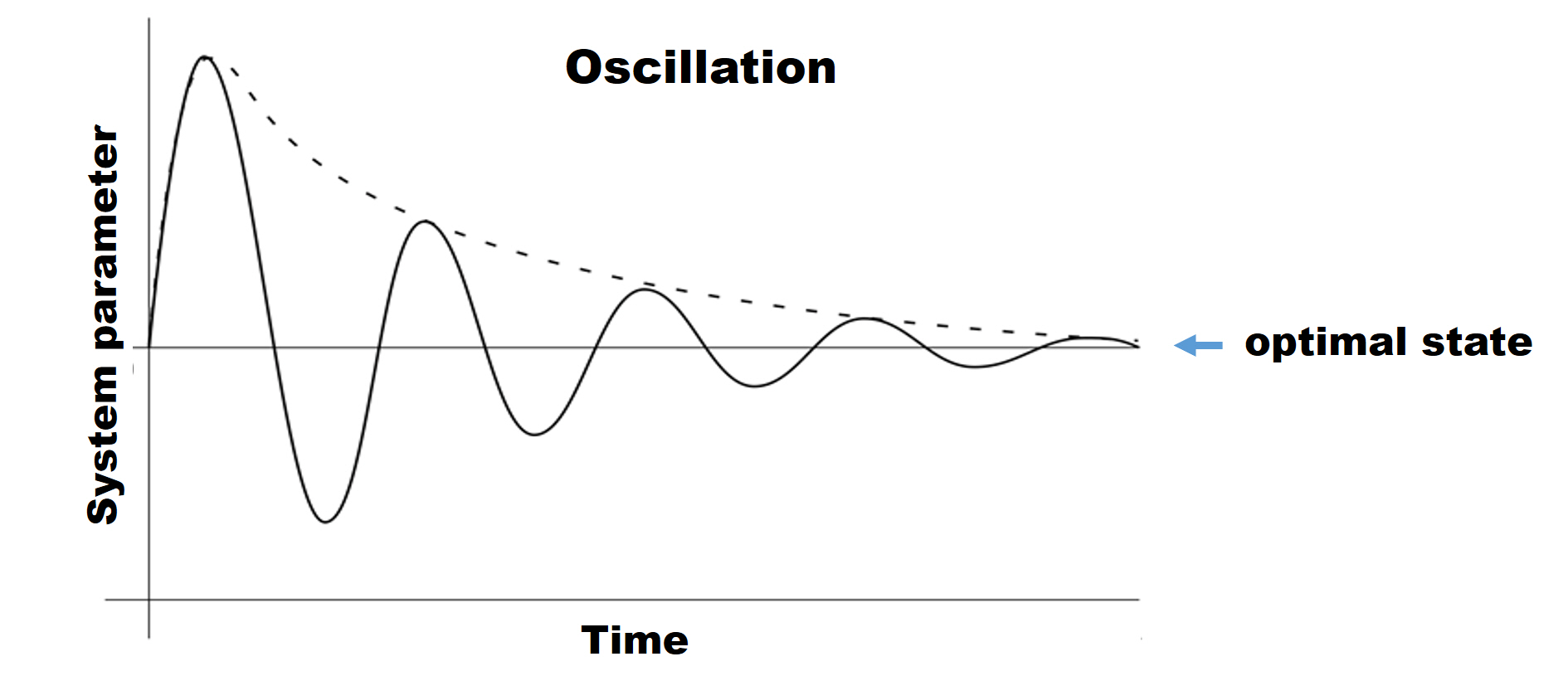
We can also depict this process in a system diagram if you wish:

Figure 1.24. Shower system diagram with water regulation feedbacks. Coldness of water draws down the comfort level and prompts the responder to adjust the knob to increase the hotness of water, which is supposed to bring the comfort level to optimal. There are two negative feedback loops that help stabilize the system. However, the delay in the couplings between the knob adjustment and actual hotness of water felt by the person (shown by red marks) results in the adjustments being disproportional with the anticipated temperature change.  

Credit: Mark Fedkin

In this process, the temperature of water goes up and down, only bypassing the optimal comfort temperature, resulting in oscillation. Eventually, understanding the delay, you start being more patient, wait for the change and make smaller adjustments. With a few more overshoots, you finally reach the optimal temperature. The system is stabilized!

Why are you able to stabilize the system eventually? In the process of regulating water temperature, you learn – you get information about how long the delay is between the knob turn and actual water temperature change. You also learn how much the temperature changes per certain degree of knob turning. Of course, you process this information almost subconsciously, and it takes a little bit of trial and error.    

 Figure 1.25. Common oscillation pattern for a parameter observed in systems that are regulated by negative feedbacks with delays.

Credit: Mark Fedkin

Many other systems with negative feedbacks – for instance, regulation of inventory stock based on supply and demand, regulation of earth climate by biota – may exhibit similar oscillations that complicate the system behavior.

Very often, regulating the system operation to improve its performance comes down to managing its delays. Interestingly, acting fast in the system with delays may only exacerbate the situation and make negative impacts and further delays even more dramatic. Instead, understanding delays and letting them run their course may be a better strategy to optimize system performance [Eakes, 2018].  

Tipping points

Tipping points is another interesting phenomenon that occurs in some systems. This topic can certainly be a subject for a deeper discussion, but it is worth mentioning it here at least briefly.

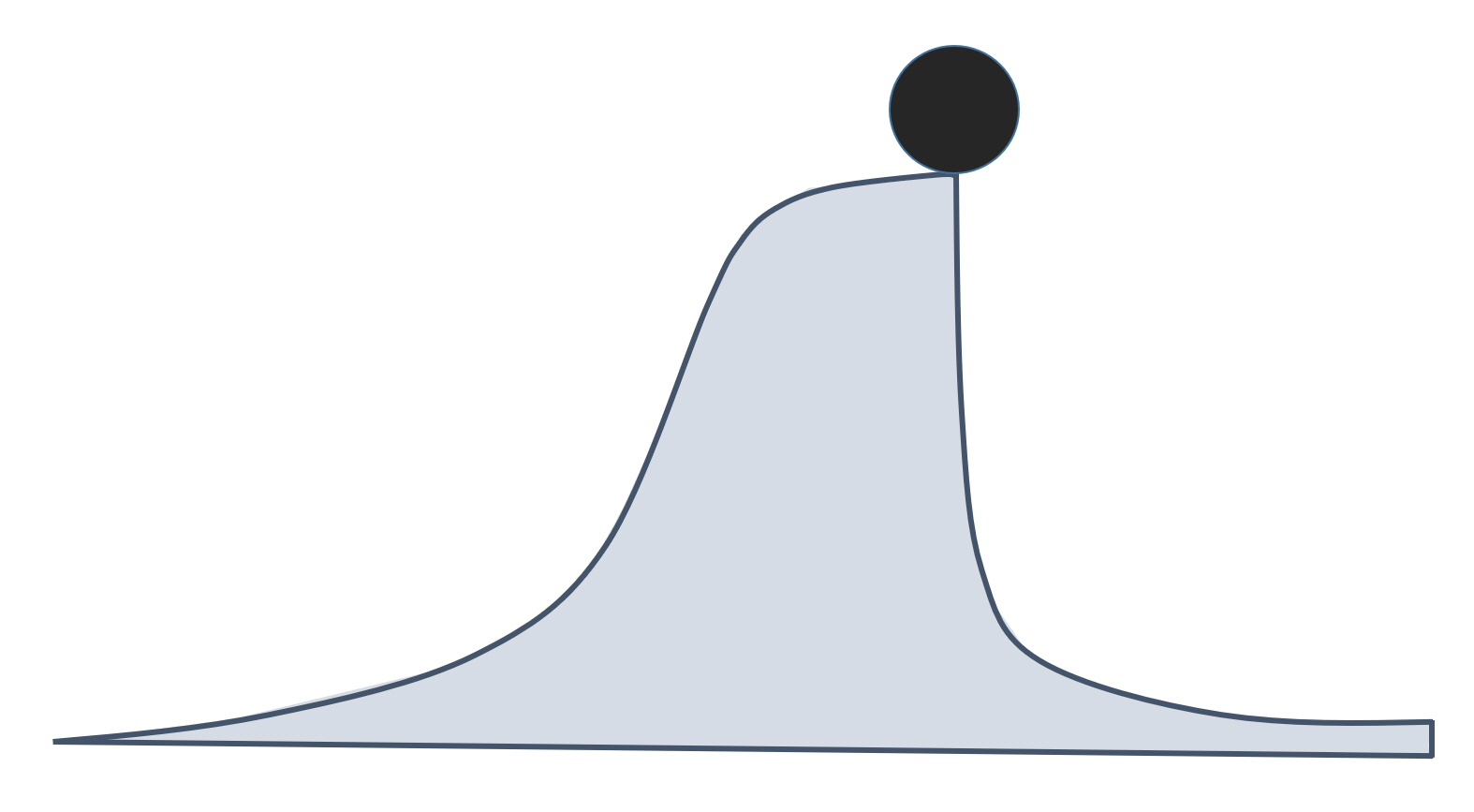
Tipping point is a special condition in a system, at which a very small perturbation or causes a large or even catastrophic change. Obviously, the small change is not the main cause, but only a trigger, the last drop in a long and sometimes complicated chain of interactions and events that lead the system to this condition. The term “tipping point” originated in the mathematical catastrophe theory and only recently started to be used in the global environmental context. Most frequently, tipping points are investigated in the relation to climate science and ecology.

Tipping points are frightening because they are not easily predictable, and when the tipping events are triggered, there is no way to reverse the process. Also the events that occur when a system passes through a tipping point are usually dramatic, proceed at a high rate, and have no forewarning. Therefore, understanding the nature and the actual causes behind the tipping points is important for designing preventive measures. Tipping points are very characteristic of systems with counteracting negative and positive feedbacks.

If you are compelled to read more about this concept, additional explanations and some good examples are given in the following reading:

It should be understood that tipping points are not results of external forces, which can also cause dramatic shifts and catastrophes, but are rather internally justified. Another take-away is that, like any other systemic phenomena, tipping points can happen in both natural and social worlds – they are not only confined to the physical processes. Tipping points are observed in societal systems and can be marked by major paradigm shifts, dramatic changes in thinking, decision making, and political transformations. It is very possible that passing of the human society from the current state to a new state with a higher degree of sustainability may also require passing through a tipping point when some traditional worldviews are rejected, and new ones are adopted. Hence, the tipping points do not only present risks, but also opportunities in socio-economic evolution.   

Boundaries and system hierarchy

It should be noted that any system model is always a simplification, and system analysis has to be iterative to identify the most significant controls and relationships that determine system operation and stability. Although limited, system analysis can provide interesting insights into system behavior, helps understand the trends in social and technological development, and provides grounds for short-term and long-term predictions.

While real systems are often complicated, making the system model overly complex is not practical - it is important to set boundaries, which would help constrain the analysis and provide answers to practical questions. Boundaries are defined by the observer. Boundaries do not mean that the system is isolated from the outer world, they simply set limits; any entities beyond system boundaries are assumed to be of minor relevance and are not examined in detail until the current model requires. For example, in the honey bee hive system described earlier, we do not consider the factor of climate, even though it is important. In the short term analysis, we simply assume it is constant. Also, we do not include economic factors such as the honey market or artificial beekeeping, etc., leaving them outside the system boundaries and just focusing on the health of the natural ecosystem.

Virtually any system is a hierarchy. That means that any system consists of smaller subsystems, and any system, in turn, may be considered as an element of a bigger system. The tree itself is a system; the soil bed is a system; any biological organism is a system with its own control factors. At the same time, the forest can be considered as a sub-system of eco-region, which is, in turn, may be perceived as a sub-system of the planet, etc. This is another reason for setting boundaries and choosing system scale before engaging in system analysis.