
6.4. Inverters: principle of operation and parameters
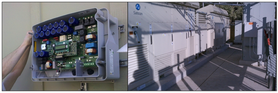
Now, let us zoom in and take a closer look at the one of the key components of power conditioning chain - inverter. Almost any solar systems of any scale include an inverter of some type to allow the power to be used on site for AC-powered appliances or on the grid. Different types of inverters are shown in Figure 11.1 as examples. The available inverter models are now very efficient (over 95% power conversion efficiency), reliable, and economical. On the utility scale, the main challenges are related to system configuration in order to achieve safe operation and to reduce conversion losses to a minimum.
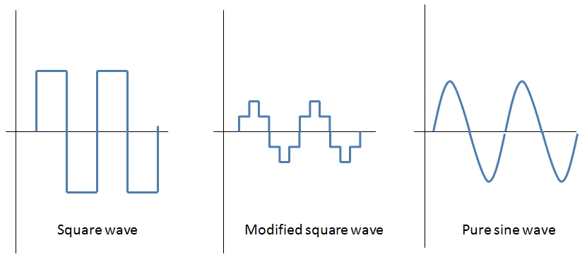
The three most common types of inverters made for powering AC loads include: (1) pure sine wave inverter (for general applications), (2) modified square wave inverter (for resistive, capacitive, and inductive loads), and (3) square wave inverter (for some resistive loads) (MPP Solar, 2015). Those wave types were briefly introduced in Lesson 6 (Figure 11.2). Here, we will take a closer look at the physical principles used by inverters to produce those signals.
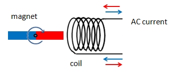
The process of conversion of the DC current into AC current is based on the phenomenon of electromagnetic induction. Electromagnetic induction is the generation of electric potential difference in a conductor when it is exposed to a varying magnetic field. For example, if you place a coil (spool of wire) near a rotating magnet, electric current will be induced in the coil (Figure 11.3).
Next, if we consider a system with two coils (Figure 11.4) and pass DC current through one of them (primary coil), that coil with DC current can act analogously to the magnet (since electric current produces a magnetic field). If the direction of the current is reversed frequently (e.g., via a switch device), the alternating magnetic field will induce AC current in the secondary coil.
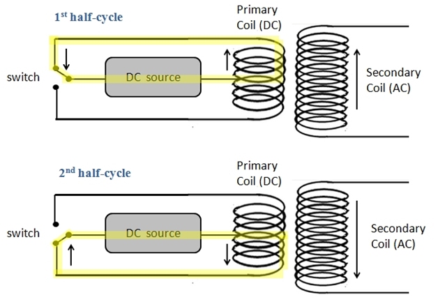
The simple two-cycle scheme shown in Figure 11.4 produces a square wave AC signal. This is the simplest case, and if the inverter performs only this step, it is a square-wave inverter. This type of output is not very efficient and can be even detrimental to some loads. So, the square wave can be modified further using more sophisticated inverters to produce a modified square wave or sine wave (Dunlop, 2010).
To produce a modified square wave output, such as the one shown in the center of Figure 11.2, low frequency waveform control can be used in the inverter. This feature allows adjusting the duration of the alternating square pulses. Also, transformers are used here to vary the output voltage. Combination of pulses of different length and voltage results in a multi-stepped modified square wave, which closely matches the sine wave shape. The low frequency inverters typically operate at ~60 Hz frequency.
To produce a sine wave output, high-frequency inverters are used. These inverters use the pulse-width modification method: switching currents at high frequency, and for variable periods of time. For example, very narrow (short) pulses simulate a low voltage situation, and wide (long pulses) simulate high voltage. Also, this method allows spacing the pulses to be varied: spacing narrow pulses farther apart models low voltage (Figure 11.5).
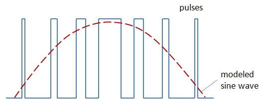
In the image above, the blue line shows the square wave varied by the length of the pulse and timing between pulses; the red curve shows how those alternating signals are modeled by a sine wave. Using very high frequency helps create very gradual changes in pulse width and thus models a true sine signal. The pulse-width modulation method and novel digital controllers have resulted in very efficient inverters (Dunlop, 2010).