Part II: Create Habitat Quality and Forest Patch Datasets
In Part II, we will use the roads dataset to create raster data layers of habitat quality and forest patches. In Part III, we will generate statistics about the size, shape, and habitat quality of each forest patch.
We will use the following coded values:
- 1- Low Quality Habitat (Road Clearings)
- 2- Medium Quality Habitat (Forest, Edge Habitat)
- 3- High Quality Habitat (Forest, Interior Habitat)
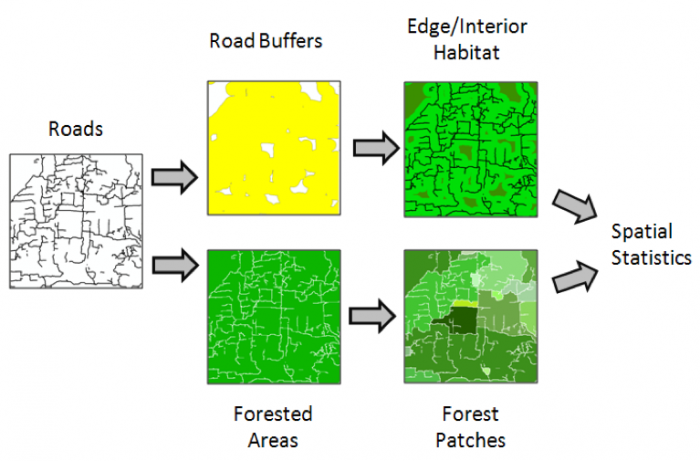 Road Dataset Flow ChartClick here for an accessible text alternative to the image aboveRoads → Road Buffers → Edge/Interior Habitat → Spacial Statistics Roads → Forested Areas → Forest Patches → Spacial Statistics
-
Create Grid of Low-Quality Habitat (Road Clearings)
- Open the "Roads07" attribute table and add a new short integer field named "HabitatCode." Save your changes.
- Use the Calculate Field tool to assign all of the roads a HabitatCode of "1." Clear the selected records.

When you convert a feature layer to a raster, you have to choose a field in the feature layer from which to base the grid cell values on. You often need to create a new dummy field and assign a value that is consistent for all of the records you want to convert (like we did above).
It is also important to note that if there are any selected records in the vector layer, only those records will be converted to a raster layer. Therefore, be sure to clear any selected features before performing the conversion.
The data type of the field you choose is very important. For example, if you choose a numerical field that contains decimal values, the resultant grid will not have an attribute table. However, if you choose an integer field, the resultant raster will have an attribute table. If you choose a text field, ArcGIS will automatically assign each unique text value an integer code in a new field named "VALUE."
The new raster layer will be created based on all defined Spatial Analyst environment settings. Always check these settings before converting features to a raster to avoid potentially undesirable results.
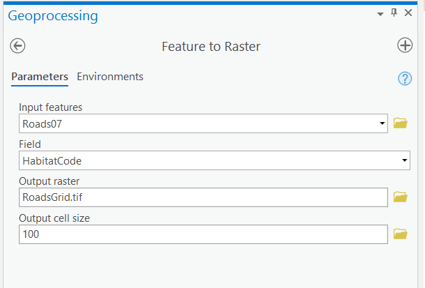
- Convert the roads feature class to a raster named "RoadsGrid.tif" using the settings below: Analysis > Tools > Toolboxes > Conversion Tools > To Raster > Feature to Raster.
- Click Run. Compare the "RoadsGrid.tif" to the road centerlines. Make sure you zoom to several different scales. Open the "RoadsGrid.tif" attribute table to view the results.
It is important to note that although the extent setting is utilized by Feature to Raster, the mask setting is ignored. Although you will not notice this with the "RoadsGrid.tif" layer, you will see the effects of this when you create a buffered grid later in this lesson.

Make sure you have the correct answer before moving on to the next step.
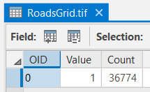
The "RoadsGrid.tif" raster should have the following information. If your data does not match this, go back and redo the previous step.
-
Create Edge Effects Grid
Remember from the Background Information section that edge effects can occur up to 2 km from roads. We will consider all areas 2 km from roads as "edge habitat" and areas farther than 2 km from roads as "interior habitat." To do this, we need to create a buffer of the road centerlines.
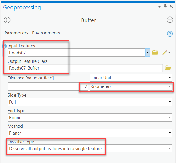
- Create a 2 km buffer of the road centerlines. Go to the Analysis tab, within the Tools group and click Buffer
 . Using the settings specified in red boxes below (allow other settings to default). Save the file inside the Lesson 7 geodatabase.
Click Run.
. Using the settings specified in red boxes below (allow other settings to default). Save the file inside the Lesson 7 geodatabase.
Click Run.
- Compare the buffer to the road centerlines. You may want to use the measuring tool to double check your buffer is the correct width.
- Add a new short integer field named "HabCode" to the "Roads07_Buffer" feature class and assign it a value of "2" using the field calculator. The value of "2" corresponds to medium quality habitat (forested areas within 2 km of a road).
- Convert the road buffer to a grid named "EdgeGrid.tif" based on the "HabCode" field. Be sure to pay attention to the cell size.
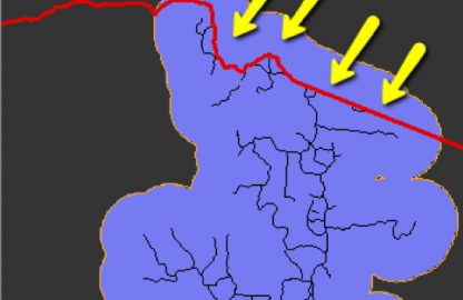
- Compare the "EdgeGrid.tif raster to the "Roads07" and "Roads07_Buffer" datasets. Notice how the conversion tool did not follow the mask setting, as the raster cells with values extrude beyond the study area boundary. It may be easier to see the effect if you assign values of NoData in the EdgeGrid raster a color as we did in previous lessons.
Make sure you have the correct answer before moving on to the next step.
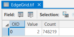
The "EdgeGrid" raster should have the following information. If your data does not match this, go back and redo the previous step.
- Create a 2 km buffer of the road centerlines. Go to the Analysis tab, within the Tools group and click Buffer
-
Create Interior Forests Grid
- Open the "Study_Boundary" attribute table and add a new short integer field named "Value." Save your changes.
- Use the Calculate Field tool to assign a Value of "1" to the study boundary.
- Convert the Study_Boundary feature class to a raster named "Study_Boundary.tif" using the Value field and an output cell size of 100: Analysis > Tools > Toolboxes > Conversion Tools > To Raster > Feature to Raster.
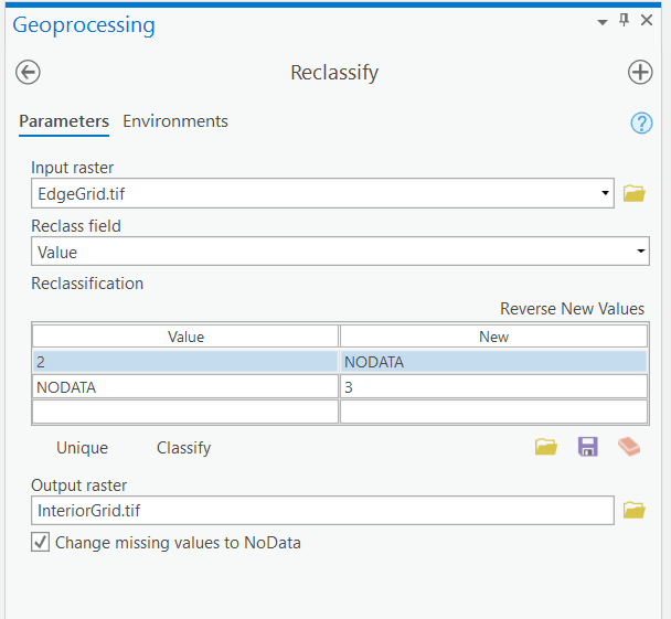
- Reclassify the "EdgeGrid.tif" and use the "Study_Boundary.tif" as the mask. See the other settings below. Name the output grid "InteriorGrid.tif" and click Run.
- Compare the "InteriorGrid.tif" raster layer to the "EdgeGrid.tif" and "RoadsGrid.tif" layers. Notice how we were able to "flip" the areas with NoData. It is easier to see the effect if you turn off all of the layers except the Roads, InteriorGrid, and Study Boundary. It’s important that you choose appropriate mask and extent settings when using this technique.

Did the Reclassify Tool honor the mask and extent settings?
Hint: Compare the InteriorGrid.tif and EdgeGrid.tif rasters along the study area boundary.
Make sure you have the correct answer before moving on to the next step.
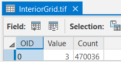
The "InteriorGrid.tif" grid should have the following information. If your data does not match this, go back and redo the previous step.
-
Create Final Habitat Quality Grid
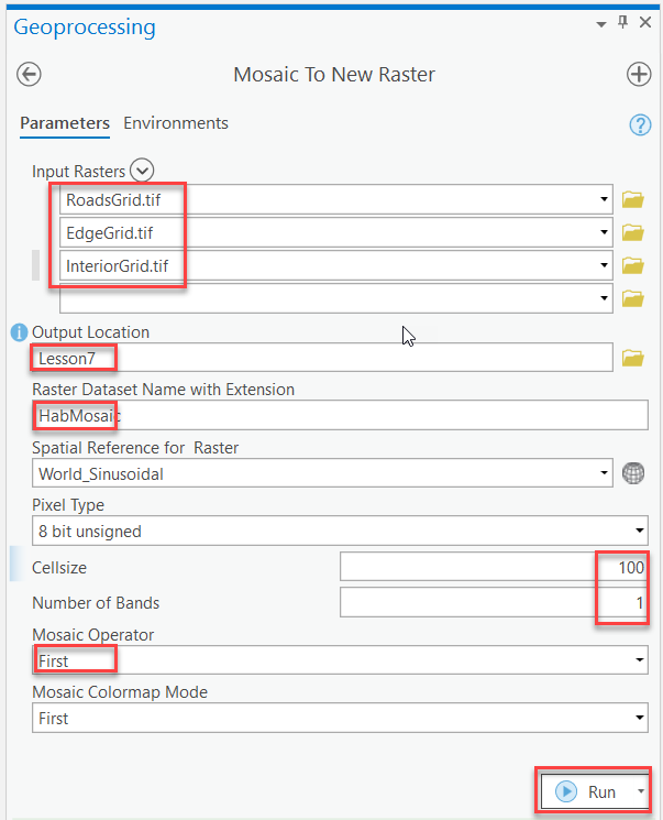
In steps 1, 2, and 3, we created three individual grids, one for each level of habitat quality. To continue the analysis, we need a way to merge all of the data sets into one grid. The Mosaic to New Raster tool in Toolboxes will allow you to mosaic multiple raster data layers together by stacking them on top of one another. The values in the output raster will be determined based on the order the files are specified during the mosaic. Cells will first be assigned according to the cell values in the first input raster; all remaining null values will be filled in with the middle input raster, and so on. We want the roads to be on top of the stack, the edge habitat in the middle, and the forests on the bottom.
- Go to the Analysis tab, Geoprocessing group and select Tools > Toolboxes > Data Management Tools > Raster > Raster Dataset > Mosaic to New Raster and enter the settings as shown below. Name the new grid "HabMosaic" and save it to your L7 folder. When adding the input rasters, pay attention to the order in which you add them. Along with the output location and the raster dataset name, you will need to assign a cell size and number of bands. The number of bands refers to a color map. Since we are not dealing with multiple band data, enter "1" to identify the new raster dataset as a single band layer. As mentioned above, we want the raster to be created based on a hierarchy from first to last. Therefore, we need to set the Mosaic Operator to "FIRST" so that the analysis runs as intended. You can leave the Mosiac Colormap Mode setting to "FIRST" since we are dealing with single-band data.
This tool does not honor the Output extent environment settings. If you want a specific extent for your output raster, consider using the Clip tool. You can either clip the input rasters prior to using this tool, or clip the output of this tool.
Make sure you have the correct answer before moving on to the next step.
The "HabMosaic" raster should have the following information. If your data does not match this, go back and redo the previous step.
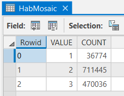
What value was assigned to areas with roads, since they have data in both the "RoadsGrid" and "EdgeGrid" rasters?
Which habitat type (roads, edge, or interior) covers the majority of the study area?
How can you calculate the area of each habitat type?
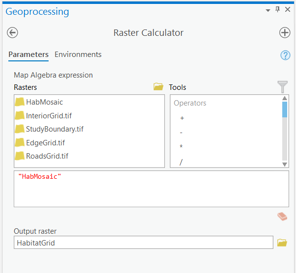
- Notice that some edges of the "HabMosaic" grid fall outside of the study boundary. As mentioned earlier, this is because the Mosaic to New Raster tool does not utilize the environments extent setting. Therefore, we need to "clip" the data to the extent of our study boundary. To do this, we will use the Raster Calculator. Open the Raster Calculator (Toolboxes > Spatial Analyst Tools > Map Algebra > Raster Calculator), click the "HabMosaic" grid to enter it into the expression window, set the output raster as "HabitatGrid" and click OK to run the expression.
- Compare the "HabitatGrid" to the "HabMosaic" grids to see how the Raster Calculator "clipped" the data. Hint: Zoom into the study area boundary,
The Raster Calculator utilizes all raster environment settings, so it is highly useful when working with raster data. As displayed above, simply selecting a raster layer and running the Raster Calculator will generate a new raster layer based on the current environmental settings. Try changing these settings to see the differences when running the Raster Calculator on a particular raster layer.
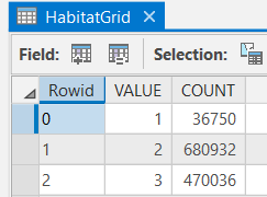
Make sure you have the correct answer before moving on to the next step.
The "HabitatGrid" raster should have the following information. If your data does not match this, go back and redo the previous step.
- Go to the Analysis tab, Geoprocessing group and select Tools > Toolboxes > Data Management Tools > Raster > Raster Dataset > Mosaic to New Raster and enter the settings as shown below. Name the new grid "HabMosaic" and save it to your L7 folder. When adding the input rasters, pay attention to the order in which you add them. Along with the output location and the raster dataset name, you will need to assign a cell size and number of bands. The number of bands refers to a color map. Since we are not dealing with multiple band data, enter "1" to identify the new raster dataset as a single band layer. As mentioned above, we want the raster to be created based on a hierarchy from first to last. Therefore, we need to set the Mosaic Operator to "FIRST" so that the analysis runs as intended. You can leave the Mosiac Colormap Mode setting to "FIRST" since we are dealing with single-band data.
-
Create Grid of Forested Areas
We now have one grid with values showing the range of habitat quality within the study area. The next step is to create a grid of forested areas, which we need to create the forest fragments. We will use the "RoadsGrid.tif" raster we created in Part II Step 1 to create a new grid representing forested areas (cells that are NOT roads).
- Reclassify "RoadsGrid.tif" using the settings below:
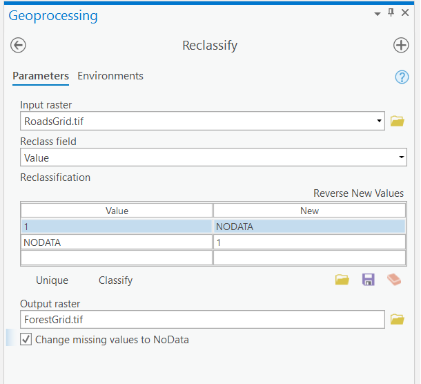
- Compare the "ForestGrid.tif" raster to the "RoadsGrid.tif" raster.
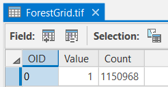
Make sure you have the correct answer before moving on to the next step.
The "ForestGrid.tif" raster should have the following information. If your data does not match this, go back and redo the previous step. You may need to adjust for the Mask and Processing Extent here as well.
- Reclassify "RoadsGrid.tif" using the settings below:
-
Create Grid of Individual Forest Patches
- Examine the "ForestGrid.tif" attribute table. Notice there is not a way to distinguish groups of contiguous cells from one another. We need to be able to do this to determine which cells belong to the same forest patch.
- To accomplish this, we will use the RegionGroup tool. RegionGroup is an operation that takes adjacent cells with the same value and assigns them a unique value. So, in essence, it creates a grid with groups of cells similar to polygons in a feature class layer. This is an important operation since it enables further analysis with expressions and operations that require grouped regions, such as calculating the area and width of forest patches.
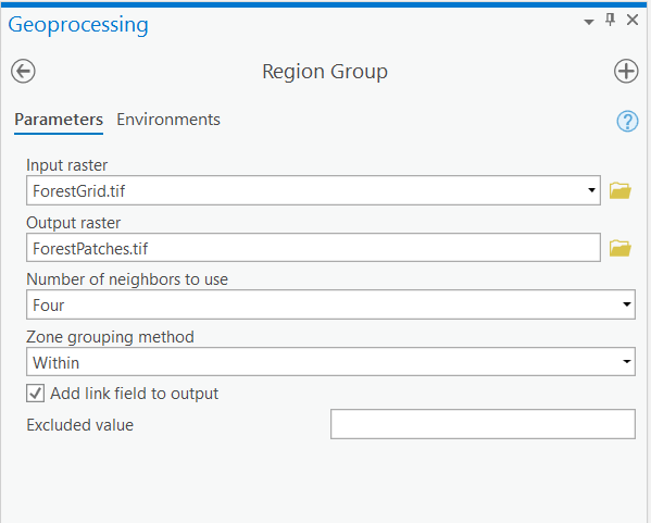
- Go to Toolboxes > Spatial Analyst Tools > Generalization > Region Group, select "ForestGrid.tif" as the input raster, name the output raster "ForestPatches.tif", leave the number of neighbors to use as "FOUR", the zone grouping method as "WITHIN", leave the link and excluded value setting, and click Run.
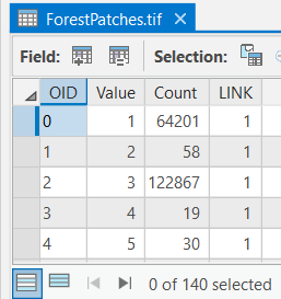
- Compare the ForestPatches.tif attribute table to the ForestGrid.tif attribute table. Notice how the attribute table now has multiple rows, one for each forest patch. The "Rowid" and "VALUE" fields both contain unique ID numbers for each contiguous forest patch. The "COUNT" field shows the number of cells in each forest patch.
Make sure you have the correct answer before moving on to the next step.
The "ForestPatches.tif" grid should have the following information. If your data does not match this, go back and redo the previous step.
 Click here for an accessible version of the image above
Data to Compare your results to OID Value Count link 0 1 64201 1 1 2 58 1 2 3 122867 1 3 4 19 1 4 5 30 1 - The "VALUE" field is very important since it uniquely identifies each forest patch. However, the default name assigned by the computer is not very meaningful. It would be very easy to forget what it means later on. It’s also easy to confuse the "VALUE" and "Rowid" field since they contain similar numbers.
- To prevent these issues, let’s create a more meaningful attribute to keep track of the forest patches. Add a new short integer field named "ForestID" to the "ForestPatches.tif" attribute table. Populate it with the numbers in the !VALUE! field.
- Change the symbology to "unique values" based on the "ForestID" field. Notice how groups of contiguous cells are now considered one unit. Also, notice how the default colors assigned by ArcGIS are not very meaningful. We will address this later in the lesson.
- The "COUNT" field is also very important since it tells us how many cells are within each forest patch. As we saw in Lesson 5, we can use the number of cells and the size of each cell to calculate area values.
- Add a new float field to the "ForestPatches.tif" attribute table named "AREA_SQM." Use the calculate field tool to populate the field.
You can also delete the Link field.
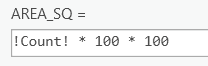
Why did we use the number "100" to calculate the area?
Make sure you have the correct answer before moving on to the next step.
The "ForestPatches.tif" grid should have the following information. If your data does not match this, go back and redo the previous step.
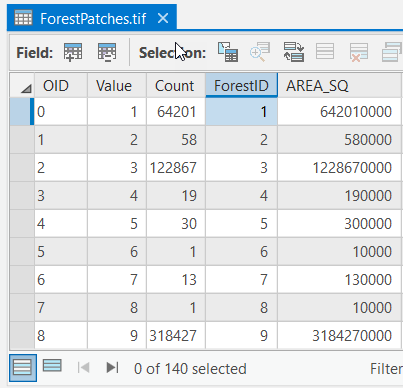 Click here for an accessible version of the image above
Data Values to Compare To oid value count forestid area_sq 0 1 64201 1 642010000 1 2 58 2 580000 2 3 122867 3 1228670000 3 4 19 4 190000 4 5 30 5 300000 5 6 1 6 10000 6 7 13 7 130000 7 8 1 8 10000 8 9 318427 9 3184270000 How many individual forest patches are there? Which forest patch is the largest? Which forest patch is the smallest? Why do you think there are so many patches with an area of exactly 10,000 sq m?