Part III: Calculate Spatial Statistics of Forest Patches
In Part III, we will use two Spatial Analyst tools to bring together the raster layers we created in Part I (habitat quality) and Part II (forest patches). Zonal Geometry calculates several geometry measures, such as area and thickness, for zones in a raster. We will use it to generate a table of statistics about the size and shape of each forest patch. We will also use the Zonal Histogram Tool to tabulate the number of cells of each habitat type within each forest patch and management unit.
-
Calculate the Geometry of Each Forest Patch
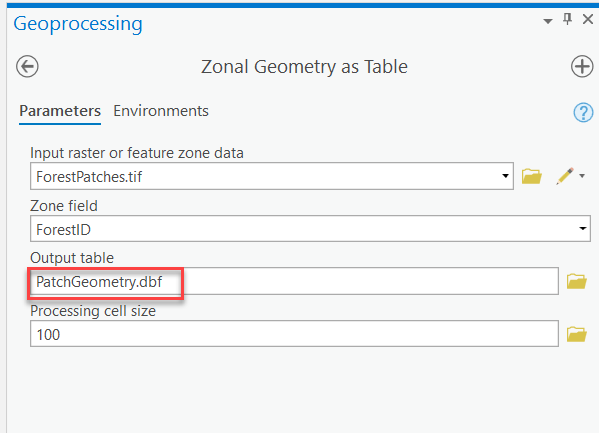
- Go to Toolboxes > Spatial Analyst Tools > Zonal > Zonal Geometry as Table. Use the settings shown below. Name the table "PatchGeometry.dbf" and save it in your Lesson7 folder. Make sure to include the .dbf file extension.

Make sure you have the correct answer before moving on to the next step.
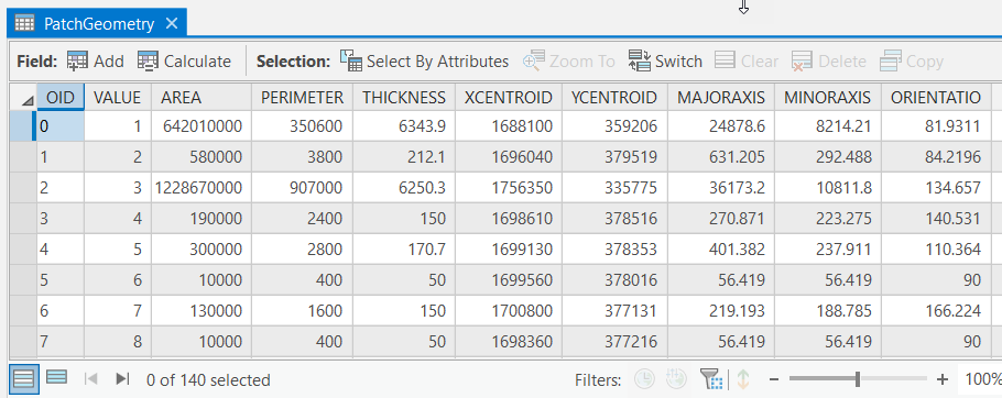
The "PatchGeometry" table should have the following information. If your data does not match this, go back and redo the previous step.
 Click here for an accessible alternative to the image above
Accessible PatchGeometry Data Set OID Value Area Perimeter Thickness Xcentroid ycentroid Majoraxis minoraxis orientation 0 1 642010000 350600 6343.9 1688100 359206 24878.6 8214.21 81.9311 1 2 580000 3800 212.1 1696040 379519 631.205 292.488 84.2196 2 3 1228670000 907000 6250.3 1756350 335775 36173.2 10811.8 134.675 3 4 190000 2400 150 1698610 378516 270.871 223.275 140.531 4 5 300000 2800 170.7 1699130 378353 401.382 237.911 110.363 5 6 10000 400 50 1699560 378016 56.419 56.419 90 6 7 130000 1600 150 1700800 377131 219.193 188.785 166.224 7 8 10000 400 50 1698360 377216 56.419 56.419 90 
Which field in the "PatchGeometry" table is the equivalent to the "ForestID" field? What are the units of the fields "AREA," "PERIMETER," and "THICKNESS"? What do the values in the fields "XCENTROID," "YCENTROID," "MAJORAXIS," "MINORAXIS", and "ORIENTATION" mean?
- Add a new short integer field named "ForestID" and populate it with the values in the "VALUE" field using the field calculator. This step will make it easier to compare the Patch Geometry table with other outputs later in the lesson.
- Add three new float fields named “TotAreaSQM,” “PerimeterM", and “ThicknessM.” Calculate them to equal the values in “AREA,” "PERIMETER,” and "THICKNESS,” respectively. This will help us remember the units of the calculations later on.
- Go to Toolboxes > Spatial Analyst Tools > Zonal > Zonal Geometry as Table. Use the settings shown below. Name the table "PatchGeometry.dbf" and save it in your Lesson7 folder. Make sure to include the .dbf file extension.
-
Calculate Habitat Statistics by Forest Patch
The Zonal Histogram tool will create a summary table that contains one row for each unique value in the "Value raster" and one column for each unique value in the "Zone dataset." The tool will calculate the total number of cells for each combination of a unique row and column. The tool can also create a graph based on the output table, which we are going to skip.
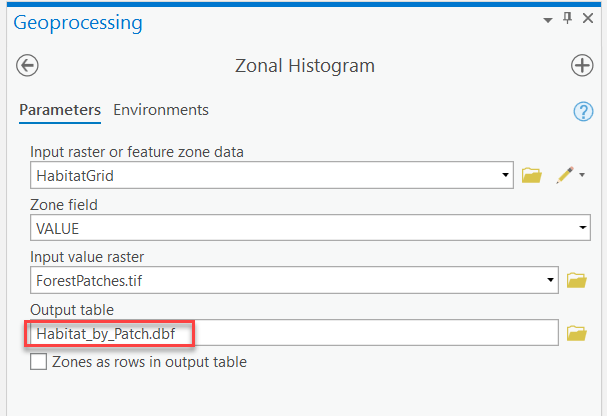
- Open the Zonal Histogram tool (Toolboxes > Spatial Analyst Tools > Zonal > Zonal Histogram). Use the settings below and click "Run." Make sure to add the .dbf extension.
- Open the "Habitat_by_Patch" table. The "LABEL" field contains values equivalent to the "Rowid" field within "ForestPatches." The "VALUE_2" field contains the number of cells of edge habitat for each forest patch. The "VALUE_3" field contains the number of cells of interior habitat for each forest patch (Remember that we used codes of 1, 2, and 3 to represent the different habitat types throughout the lesson).
- These field names are not very intuitive, and we may forget what they mean later on. Let’s add a few new meaningful fields to address this potential problem.
- Add a new short integer field called "ForestID" to the "Habitat_by_Patch" table. Use the calculate field tool to populate it with the values in the “LABEL” field.
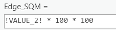
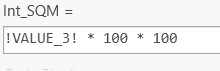
- Add two new float fields named "Edge_SQM" and "Int_SQM." Calculate the fields as shown below (# of cells * cell length * cell width):
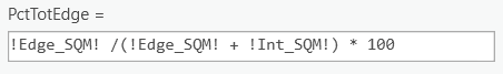
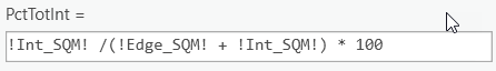
- Remember from Lesson 4 that it is a lot easier to compare multiple area values if you use percent of the total area instead of actual area values. Add two new short integer fields named "PctTotEdge" and "PctTotInt." Calculate the fields as shown below. Notice the 100 in the equation is used to create a percent value and is not related to the 100 value we used in step e, which corresponds to the length and width of the raster cells.
Make sure you have the correct answer before moving on to the next step.
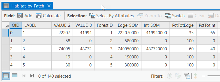
The "Habitat_by_Patch" table should have the following information. If your data does not match this, go back and redo the previous step.
 Click here for an accessible alternative to the image above
Accessible Habitat_by_Patch Data Set oid Label Value_2 Value_3 FORESTID EDge_sqm int_sqM PCTtotedge pcttotint 0 1 22207 41994 1 222070000 419940000 35 65 1 2 58 0 2 580000 0 100 0 2 3 74095 48772 3 740950000 487720000 60 40 3 4 19 0 4 190000 0 100 0 4 5 30 0 5 300000 0 100 0
- Open the Zonal Histogram tool (Toolboxes > Spatial Analyst Tools > Zonal > Zonal Histogram). Use the settings below and click "Run." Make sure to add the .dbf extension.
-
Calculate Habitat Statistics by Management Unit
- Use the Zonal Histogram Tool to determine the amount of each habitat type by management unit as shown in the example below: Don’t forget the file extension.
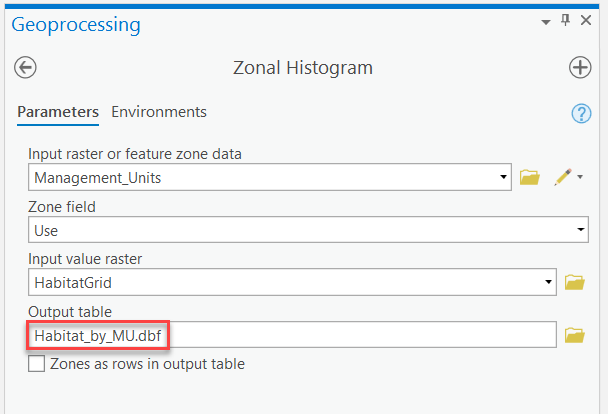
What do numbers in the "LABEL" field of the "Habitat_by_MU" mean? Which management unit "use" has the most roads?
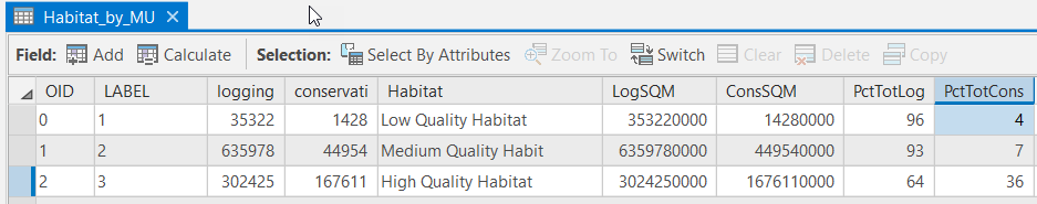
- Add a new text field (length 25) named “Habitat.” Use the field calculator and the information below to update the new field.
- 1 - Low-Quality Habitat (Road Clearings)
- 2 - Medium Quality Habitat (Forest, Edge Habitat)
- 3 - High-Quality Habitat (Forest, Interior Habitat)
- Add two new float fields named “LogSQM” and “ConsSQM.” Add two new short integer fields named “PctTotLog” and “PctTotCons.” Calculate them using the technique we used in Step 2 e and f.
Make sure you have the correct answer before moving on to the next step.
The "Habitat_by_MU" table should have the following values. If your data does not match this, go back and redo the previous step.
 Click here for an accessible alternative to the image above
Accessible Habitat_by_MU dataset OID Label logging coservation habitat logSqm conssqm pcttotlog pcttotcons 0 1 35322 1428 Low Quality Habitat 353220000 14280000 96 4 1 2 635978 44954 Medium Quality Habitat 6359780000 449540000 93 7 2 3 302425 167611 High Quality Habitat 3024250000 1676110000 64 36 -
Join Forest Patches to Geometry Table
- Since we no longer need the forest patches to be in raster format, let’s convert them to a shapefile so they are easier to use.
- Convert the "ForestPatches.tif" grid to a polygon shapefile using the settings below: Toolboxes > Conversion Tools > From Raster > Raster to Polygon.
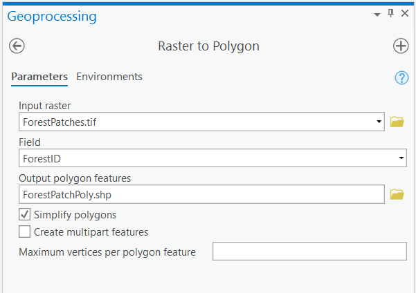
- Add a new short integer field named "FORESTID" and populate it with the values in the "GRIDCODE" field.
Make sure you have the correct answer before moving on to the next step.
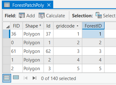
The "forestpatchpoly" shapefile should have the following information. If your data does not match this, go back and redo the previous step. Note that this table has been sorted based on "gridcode".
 Click here for an accessible alternative to the image above
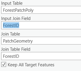
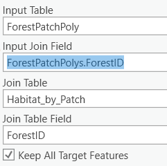
Accessible ForestPatchPoly Data Set Fid Shape* Id gridcode ForestID 36 Polygon 37 1 1 0 Polygon 1 2 2 61 Polygon 62 3 3 1 Polygon 2 4 4 2 Polygon 3 5 5 - Join the "PatchGeometry" and "Habitat_by_Patch" tables to the "forestpatchpoly" shapefile using the link fields shown below.
- Open the attribute table to make sure the joins worked properly. Notice how it is hard to view the attributes we are most interested in since there are so many fields.
- On the ribbon, go to the Table > View tab >Fields
 , and uncheck the "Visible" box on the top left side. Add the checkboxes back to the eight fields listed below and click "Save."
- ForestID
- TotAreaSQM
- PerimeterM
- ThicknessM
- Edge_SQM
- Int_SQM
- PctTotEdge
- PctTotInt
- Close and then re-open the ForestPatchPoly attribute table. Notice how it is much easier to interpret the results now.
- To make the joins and table design permanent, export the "forestpatchpoly" to a new shapefile in your Lesson 7 folder named “Final_Forest_Patches.shp.”
- Examine the attribute table.
-
Calculate the Edge to Area Ratio of each Forest Patch
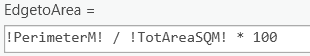
- Calculate the edge to area ratio for each patch. Add a new float field named "EdgetoArea." Calculate it as shown below. Note: we are going to multiply the result by "100" to make the values easier to compare.
Why is there such a large range of values for the edge to area ratio results?
How would the results of the analysis change if we used a larger or smaller cell size?
Make sure you have the correct answer before moving on to the next step.
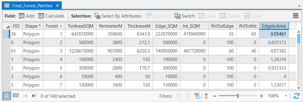
The "Final_Forest_Patches" attribute table should have the following information. If your data does not match this, go back and redo the previous step.
 Click here for an accessible alternative to the image above
Accessible Final_Forest_Patches Dataset FID Shape* Forest ID Totareasqm perimeterm thichnessm edge_sqm int_sqm pcttotedge pcttotint edgetoarea 36 Polygon 1 642010000 350600 6343.9 222070000 419940000 35 65 0.05461 0 Polygon 2 580000 3800 212.1 580000 0 100 0 0.655172 61 Polygon 3 1228670000 90700 6250.3 740950000 487720000 60 40 0.07382 1 Polygon 4 190000 2400 150 190000 0 100 0 1.26316 2 Polygon 5 300000 2800 170.7 300000 0 100 0 0.933333 3 Polygon 6 10000 400 50 10000 0 100 0 4 5 Polygon 7 130000 1600 150 130000 0 100 0 1.23077 
Notice how the default outputs from many of the Spatial Analyst tools are not very easy to understand. It’s worth the time to create more intuitive fields, units, and names while you are doing the analysis. That way you can easily interpret your results later on and share them with others in a meaningful format.
- Calculate the edge to area ratio for each patch. Add a new float field named "EdgetoArea." Calculate it as shown below. Note: we are going to multiply the result by "100" to make the values easier to compare.
- Use the Zonal Histogram Tool to determine the amount of each habitat type by management unit as shown in the example below: Don’t forget the file extension.