We will now explain the basics of editing a Jupyter Notebook. We cannot cover all the details here, so if you enjoy working with Jupyter and want to learn all it has to offer as well as all the little tricks that make life easier, the following resources may serve as good starting points:
- Jupyter Documentation
- The Jupyter Notebook
- 28 Jupyter Notebook tips, tricks, and shortcuts
- Jupyter Notebook Tutorial: The Definitive Guide
A Jupyter notebook is always organized as a sequence of so called ‘cells’ with each cell either containing some code or rich text created using the Markdown notation approach (further explained in a moment). The notebook you created in the previous section currently consists of a single empty cell marked by a blue bar on the left that indicates that this is the currently active cell and that you are in ‘Command mode’. When you click into the corresponding text field to add or modify the content of the cell, the bar color will change to green indicating that you are now in ‘Edit mode’. Clicking anywhere outside of the text area of a cell will change back to ‘Command mode’.
Let’s start with a simple example for which we need two cells, the first one with some heading and explaining text and the second one with some simple Python code. To add a second cell, you can simply click on the  symbol. The new cell will be added below the first one and become the new active cell shown by the blue bar (and frame around the cell’s content). In the ‘Insert’ menu at the top, you will also find the option to add a new cell above the currently active one. Both adding a cell above and below the current one can also be done by using the keyboard shortcuts ‘A’ and ‘B’ while in ‘Command mode’. To get an overview on the different keyboard shortcuts, you can use Help -> Keyboard Shortcuts in the menu at the top.
Both cells that we have in our notebook now start with “In [ ]:” in front of the text field for the actual cell content. This indicates that these are ‘Code’ cells, so the content will be interpreted by Jupyter as executable code. To change the type of the first cell to Markdown, select that cell by clicking on it, then change the type from ‘Code’ to ‘Markdown’ in the dropdown menu 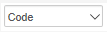 in the toolbar at the top. When you do this, the “In [ ]:” will disappear and your notebook should look similar to Figure 3.8 below. The type of a cell can also be changed by using the keyboard shortcuts ‘Y’ for ‘Code’ and ‘M’ for ‘Markdown’ when in ‘Command mode’.

Let’s start by putting some Python code into the second(!) cell of our notebook. Click on the text field of the second cell so that the bar on the left turns green and you have a blinking cursor at the beginning of the text field. Then enter the following Python code:
from bs4 import BeautifulSoup
import requests

documentURL = 'https://www.e-education.psu.edu/geog489/l1.html'

html = requests.get(documentURL).text
soup = BeautifulSoup(html, 'html.parser')

print(soup.get_text())
This brief code example is similar to what you already saw in Lesson 2. It uses the requests Python package to read in the content of an html page from the URL that is provided in the documentURL variable. Then the package BeautifulSoup4 (bs4) is used for parsing the content of the file and we simply use it to print out the plain text content with all tags and other elements removed by invoking its get_text() method in the last line.
While Jupyter by default is configured to periodically autosave the notebook, this would be a good point to explicitly save the notebook with the newly added content. You can do this by clicking the disk  symbol or simply pressing ‘S’ while in ‘Command mode’. The time of the last save will be shown at the top of the document, right next to the notebook name. You can always revert back to the last previously saved version (also referred to as a ‘Checkpoint’ in Jupyter) using File -> Revert to Checkpoint. Undo with CTRL-Z works as expected for the content of a cell while in ‘Edit mode’; however, you cannot use it to undo changes made to the structure of the notebook such as moving cells around. A deleted cell can be recovered by pressing ‘Z’ while in ‘Command mode’ though.
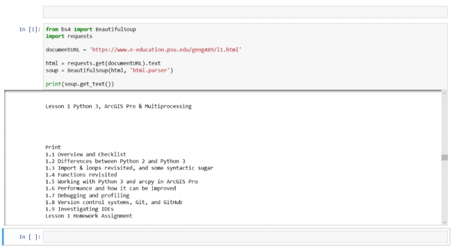
Now that we have a cell with some Python code in our notebook, it is time to execute the code and show the output it produces in the notebook. For this you simply have to click the run  symbol button or press ‘SHIFT+Enter’ while in ‘Command mode’. This will execute the currently active cell, place the produced output below the cell, and activate the next cell in the notebook. If there is no next cell (like in our example so far), a new cell will be created. While the code of the cell is being executed, a * will appear within the squared brackets of the “In [ ]:”. Once the execution has terminated, the * will be replaced by a number that always increases by one with each cell execution. This allows for keeping track of the order in which the cells in the notebook have been executed.
Figure 3.9 below shows how things should look after you executed the code cell. The output produced by the print statement is shown below the code in a text field with a vertical scrollbar. We will later see that Jupyter provides the means to display other output than just text, such as images or even interactive maps.
In addition to running just a single cell, there are also options for running all cells in the notebook from beginning to end (Cell -> Run All) or for running all cells from the currently activated one until the end of the notebook (Cell -> Run All Below). The produced output is saved as part of the notebook file, so it will be immediately available when you open the notebook again. You can remove the output for the currently active cell by using Cell -> Current Outputs -> Clear, or of all cells via Cell -> All Output -> Clear.
Let’s now put in some heading and information text into the first cell using the Markdown notation. Markdown is a notation and corresponding conversion tool that allows you to create formatted HTML without having to fiddle with tags and with far less typing required. You see examples of how it works by going Help -> Markdown in the menu bar and then clicking the “Basic writing and formatting syntax” link on the web page that opens up. This page here also provides a very brief overview on the markdown notation. If you browse through the examples, you will see that a first level heading can be produced by starting the line with a hashmark symbol (#). To make some text appear in italics, you can delimit it by * symbols (e.g., *text*), and to make it appear in bold, you would use **text** . A simple bullet point list can be produced by a sequence of lines that start with a – or a *.
Let’s say we just want to provide a title and some bullet point list of what is happening in this code example. Click on the text field of the first cell and then type in:
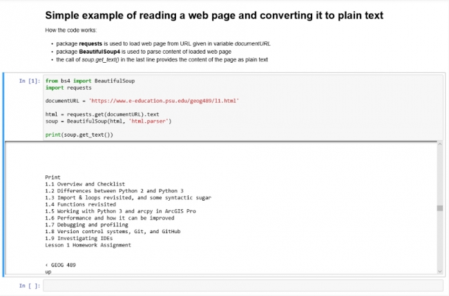
# Simple example of reading a web page and converting it to plain text
How the code works:
* package **requests** is used to load web page from URL given in variable *documentURL*
* package **BeautifulSoup4 (bs4)** is used to parse content of loaded web page
* the call of *soup.get_text()* in the last line provides the content of page as plain text
While typing this in, you will notice that Jupyter already interprets the styling information we are providing with the different notations, e.g. by using a larger blue font for the heading, by using bold font for the text appearing within the **…**, etc. However, to really turn the content into styled text, you will need to ‘run the cell’ (SHIFT+Enter) like you did with the code cell. As a result, you should get the nicely formatted text shown in Figure 3.10 below that depicts our entire first Jupyter notebook with text cell, code cell, and output. If you want to see the Markdown code and edit it again, you will have to double-click the text field or press ‘Enter’ to switch to ‘Edit mode’.
If you have not worked with Markdown styling before, we highly recommend that you take a moment to further explore the different styling options from the “Basic writing and formatting syntax” web page. Either use the first cell of our notebook to try out the different notations or create a new Markdown cell at the bottom of the notebook for experimenting.
This little example only covered the main Jupyter operations needed to create a first Jupyter notebook and run the code in it. The ‘Edit’ menu contains many operations that will be useful when creating more complex notebooks, such as deleting, copying, and moving of cells, splitting and merging functionality, etc. For most of these operations, there also exist keyboard shortcuts. If you find yourself in a situation in which you can’t figure out how to use any of these operations, please feel free to ask on the forums.