You've managed to complete your first analysis in RStudio, congratulations! As was mentioned earlier in the lesson, R also offers a notebook-like environment in which to do statistical analysis. If you'd like to try this out, follow the instructions on this page to reproduce your Lesson 2 analysis in an R Markdown file.
R Markdown: a quick overview
Since typing commands into the console can get tedious after a while, you might like to experiment with R Markdown.
R Markdown acts as a notebook where you can integrate your notes or the text of a report with your analysis. When you are finished, save the file; if you need to return to your analysis, you can load the file into R and run your analysis again. Once you have completed the analysis and write-up, you can create a final document.
Here are some resources to help you better understand RMarkdown and other tools.
- Learning tools in R
- markdown: RMarkdown cheat sheet
- markdown: RMarkdown Reference guide
- markdown: RMarkdown Tutorial
- swirl: Learn R, in R
- rcmdr: GUI for different statistical methods
Before doing anything, make sure you have installed and loaded the rmarkdown package.
 install.packages("rmarkdown")
library(rmarkdown)
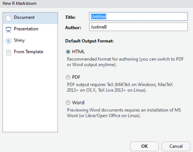
To create a new RMarkdown file, go to File – New File – R Markdown. Select the Output Format and Document. Select HTML (Figure 2.16).
Opening the RMD File and Coding
In the Lesson 2 data folder, you will find a .rmd file.
In RStudio, load the .rmd file, File – Open File. Select the Les2_crimeAnalysis.Rmd file from the Lesson 2 folder.
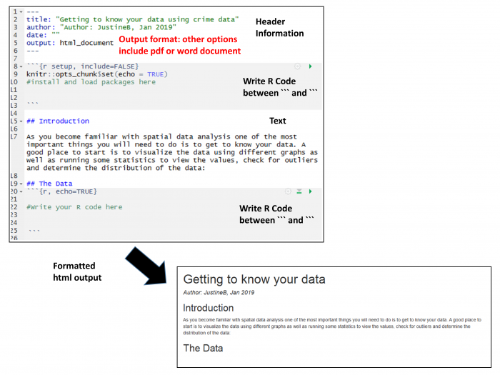
The file will open in a window in the top left quadrant of RStudio. This is essentially a text file where you can add your R code, run your analysis, and write up your notes and results.
The header is where you should add a title, date, and your name as the author. Try customizing the information there.
R code should be written in the grey areas between the ``` and ``` comments. These grey areas are called "chunks".
Note that the command {r, echo=TRUE), written at the top of each R code chunk, will include the R code in the output (see line 20 in Figure 2.17). If you do not want to include the R code, then set echo=FALSE. There are several chunk options that you can explore on your own.
include = FALSEprevents code and results from appearing in the finished file. R Markdown still runs the code in the chunk, and the results can be used by other chunks.echo = FALSEprevents code, but not the results from appearing in the finished file. This is a useful way to embed figures.message = FALSEprevents messages that are generated by code from appearing in the finished file.warning = FALSEprevents warnings that are generated by code from appearing in the finished.fig.cap = "..."adds a caption to graphical results.
Of course, setting any of these options to TRUE creates the opposite effect. Chunk options must be written in one line; no line breaks are allowed inside chunk options.
Once you have added what you need to the R Markdown file, you can use it to create a formatted text document, as shown below.
For additional information on formatting, see the RStudio cheat sheet.
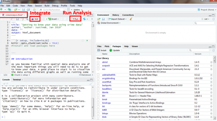
To execute the R code and create a formatted document, use Knit. Knit integrates the pieces in the file to create the output document, in this case an html_document. The Run button will execute the R code and integrate the results into the notebook. There are different options available for running your code. You can run all of your code or just a chunk of code. To run just one chunk, click the green arrow near the top of the chunk.
If you are having trouble with running just one chunk, it might be because the chunk depends on something that was done in a prior chunk. If you haven't run that prior chunk, then those results may not be available, causing either an error or an erroneous result. We recommend generally using the Knit approach or the Run Analysis button at the top (as shown in Figure 2.18).
Try the Run and Knit buttons
Note for Figure 2.18:
You probably set the output of the "knit" to HTML. Oher output options are available and can be set at the top of the markdown file.
title: "Lesson1_RMarkdownProject1doc"
author: "JustineB"
date: "January 24, 2019"
output:
word_document: default
html_document: default
editor_options:
chunk_output_type: inline
always_allow_html: yes
Add the "always_allow_html: yes" to the bottom
Your Turn!
Now you've seen how the analysis works in an R Markdown file. Try adding another chunk (Insert-R) to the R Markdown document and then copy the next blocks of your analysis code into the new chunk in the R Markdown file and then try to Knit the file. It's best to add one chunk at a time and then test the file/code by knitting it. That will make it easier to find any problems.
If you're successful, continue on until you've built out your whole R Markdown file. If you get stuck, post a description of your problem to the Lesson 2 discussion forum and ask for some help!