
In several instances, the boundaries of State Plane Coordinate Zones today, SPCS83, the State Plane Coordinate System based on NAD83 2011 (2010.0) and its reference ellipsoid GRS80, differ from the original zone boundaries. The foundation of the original State Plane Coordinate System, SPCS27 was NAD27 and its reference ellipsoid Clarke 1866. As mentioned earlier, NAD27 geographical coordinates, latitudes and longitudes, differ significantly from those in NAD83 2011 (2010.0). In fact, conversion from geographic coordinates, latitude and longitude, to grid coordinates, y and x, and back is one of the three fundamental conversions in the State Plane Coordinate system. It is important because the whole objective of the SPCS is to allow the user to work in plane coordinates, but still have the option of expressing any of the points under consideration in either latitude and longitude or State Plane Coordinates without significant loss of accuracy. Therefore, when geodetic control was migrated from NAD27 to NAD83 2011 (2010.0), the State Plane Coordinate System had to go along. When the migration was undertaken in the 1970s, it presented an opportunity for an overhaul of the system. Many options were considered, but in the end, just a few changes were made. One of the reasons for the conservative approach was the fact that 37 states had passed legislation supporting the use of State Plane Coordinates. Nevertheless, some zones got new numbers, and some of the zones changed. The zones are numbered in the SPCS83 system known as FIPS. FIPS stands for Federal Information Processing Standard, and each SPCS83 zone has been given a FIPS number. These days, the zones are often known as FIPS zones. SPCS27 zones did not have these FIPS numbers. As mentioned earlier, the original goal was to keep each zone small enough to ensure that the scale distortion was 1 part in 10,000 or less, but when the SPCS83 was designed, that scale was not maintained in some states. In five states, some SPCS27 zones were eliminated altogether and the areas they had covered were consolidated into one zone or added to adjoining zones. In three of those states, the result was one single large zone. Those states are South Carolina, Montana, and Nebraska. In SPCS27, South Carolina and Nebraska had two zones; in SPCS83, they have just one, FIPS zone 3900 and FIPS zone 2600, respectively. Montana previously had three zones. It has one, FIPS zone 2500. Therefore, because the area covered by these single zones has become so large, they are not limited by the 1 part in 10,000 standard. California eliminated zone 7 and added that area to FIPS zone 0405, formerly zone 5. Two zones previously covered Puerto Rico and the Virgin Islands. They have one. It is FIPS zone 5200. In Michigan, three Transverse Mercator zones were entirely eliminated.
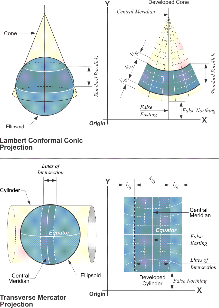
In both the Transverse Mercator and the Lambert Conic projection, the positions of the axes are similar in all SPCS zones. As you can see in the illustration, each zone has a central meridian. These central meridians are true meridians of longitude near the geometric center of the zone. Please note that the central meridian is not the y-axis. If it were the y-axis negative coordinates would result. To avoid them, the actual y-axis is moved far to the west of the zone itself. In the old SPCS27 arrangement, the y-axis was 2,000,000 feet west from the central meridian in the Lambert Conic projection and 500,000 feet in the Transverse Mercator projection. In the SPCS83 design, those constants have been changed. The most common values are 600,000 meters for the Lambert Conic and 200,000 meters for the Transverse Mercator. However, there is a good deal of variation in these numbers from state to state and zone to zone. In all cases, however, the y-axis is still far to the west of the zone and there are no negative State Plane Coordinates. No negative coordinates, because the x-axis, also known as the baseline, is far to the south of the zone. Where the x-axis and y-axis intersect is the origin of the zone, and that is always south and west of the zone itself. This configuration of the axes ensures that all State Plane Coordinates occur in the first quadrant and are, therefore, always positive.
It is important to note that the fundamental unit for SPCS27 was the U.S. survey foot, but "the U.S. survey foot will be phased out as part of the modernization of the National Spatial Reference System (NSRS). From this point forward, the international foot will be simply called the foot." https://www.nist.gov/pml/us-surveyfoot. The fundamental unit for SPCS83, it is the meter.
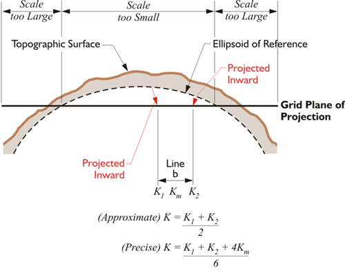
This brings us to the scale factor, also known as the K factor and the projection factor. It was this factor that the original design of the State Plane Coordinate system sought to limit to 1 part in 10,000. As implied by that effort, scale factors are ratios that can be used as multipliers to convert ellipsoidal lengths, also known as geodetic distances, to lengths on the map projection surface, also known as grid distances, and vice versa. Please notice that the geodetic distance is the distance on the ellipsoid of reference, not the distance measured on the surface of the earth. So, the geodetic length of a line, on the ellipsoid, multiplied by the appropriate scale factor will give you the grid length of that line on the state plane (the map). And the grid length multiplied by the inverse of that same scale factor would bring you back to the geodetic length again. There's another factor that will get you from topographic surface of the earth —where the measurement was made— down to the ellipsoid. However, at the moment we're talking about the scale factor. Here in this image, you see a state plane, and a horizontal line is indicated between the bases of the red arrows. Please notice that between the standard lines, the scale is too small on the state plane. And outside the standard lines, the scale is too large on the state plane. So, the line between the bases of those two red arrows on the ellipsoid of reference will be projected inward from the ellipsoid to the state plane. As it's projected inward —the line shortens. That means that between the intersection of standard lines, the grid (state plane) is under the ellipsoid. In that area, a distance from one point to another is longer on the ellipsoid than on the state plane. This means that right in the middle of the State Plane coordinate systems zone, the scale is at its minimum. In the middle, a typical minimum State Plane coordinate scale factor is not less than 0.9999. Outside of the standard lines, the grid (state plane) is above the ellipsoid where the distance from one point to another is shorter on the ellipsoid than it is on the state plane. There, at the edge of the zone, a maximum typical State Plane coordinate system scale factor is generally not more than 1.0001.
The projection used most on states that are longest from east to west is the Lambert Conic. In this projection, the scale factor for east-west lines is constant. In other words, the scale factor is the same all along the line. One way to think about this is to recall that the distance between the ellipsoid and the map projection surface does not change east to west in that projection. On the other hand, along a north-south line, the scale factor is constantly changing on the Lambert Conic. And it is no surprise then to see that the distance between the ellipsoid and the map projection surface is always changing along the north to south line in that projection. But looking at the Transverse Mercator projection, the projection used most on states longest north to south, the situation is exactly reversed. In that case, the scale factor is the same all along a north-south line, and changes constantly along an east-west line.
Both the Transverse Mercator and the Lambert Conic used a secant projection surface and originally restricted the width to 158 miles. These were two strategies used to limit scale factors when the State Plane Coordinate systems were designed. Where that was not optimum, the width was sometimes made smaller, which means the distortion was lessened. As the belt of the ellipsoid projected onto the map narrows, the distortion gets smaller. For example, Connecticut is less than 80 miles wide north to south. It has only one zone. Along its northern and southern boundaries, outside of the standard parallels, the scale factor is 1 part in 40,000, a fourfold improvement over 1 part in 10,000. And in the middle of the state, the scale factor is 1 part in 79,000, nearly an eightfold increase. On the other hand, the scale factor was allowed to get a little bit smaller than 1 part in 10,000 in Texas. By doing that, the state was covered completely with five zones. And among the guiding principles in 1933 was covering the states with as few zones as possible and having zone boundaries follow county lines. Still it requires ten zones and all three projections to cover Alaska.
When SPCS 27 was current, scale factors were interpolated from tables published for each state. In the tables for states in which the Lambert Conic projection was used, scale factors change north–south with the changes in latitude. In the tables for states in which the Transverse Mercator projection was used, scale factors change east-west with the changes in x-coordinate. Today, scale factors are not interpolated from tables for SPCS83. For both the Transverse Mercator and the Lambert Conic projections, they are calculated directly from equations. There are also several software applications that can be used to automatically calculate scale factors for particular stations. They can be used to convert latitudes and longitudes to State Plane Coordinates. Given the latitude and longitude of the stations under consideration, part of the available output from these programs is typically the scale factors for those stations. To illustrate the use of these factors, consider a line with a length on the ellipsoid of 130,210.44 feet, a bit over 24 miles. That would be its geodetic distance. Suppose that the scale factor for that line was 0.9999536, then the grid distance along the line would be:
Geodetic Distance * Scale Factor = Grid Distance
130,210.44 ft. * 0.999953617 = 130,204.40 ft.
The difference between the longer geodetic distance and the shorter grid distance here is a little more than 6 feet. That is actually better than 1 part in 20,000; please recall that the 1 part in 10,000 ratio was originally considered the maximum. Distortion lessens, and the scale factor approaches 1 as a line nears a standard parallel. Please also recall that on the Lambert projection, an east–west line, that is a line that follows a parallel of latitude, has the same scale factor at both ends and throughout. However, a line that bears in any other direction will have a different scale factor at each end. A north–south line will have a great difference in the scale factor at its north end compared with the scale factor of its south end.
Where K is the scale factor for a line, K1 is the scale factor at one end of the line and K2 is the scale factor at the other end of the line. Scale factor varies with the latitude in the Lambert projection. For example, suppose the point at the north end of the 24-mile line is called Stormy and has a geographic coordinate of:
37º46’00.7225”
103º46’35.3195”
and at the south end the point is known as Seven with a geographic coordinate of:
37º30’43.5867”
104º05’26.5420”
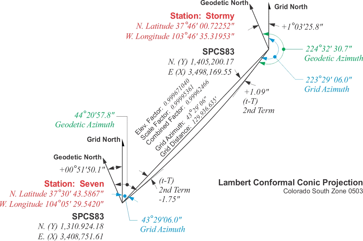
The scale factor for point Seven is 0.99996113 and the scale factor for point Stormy is 0.99994609. It happens that point Seven is further south and closer to the standard parallel than is point Stormy, and it therefore follows that the scale factor at Seven is closer to 1. It would be exactly 1 if it were on the standard parallel, which is why the standard parallels are called lines of exact scale. The typical scale factor for the line is the average of the scale factors at the two end points:
Deriving the scale factor at each end and averaging them is the usual method for calculating the scale factor of a line. The average of the two is sometimes called Km.
However, it can also be done by the precise method K = K1 + K2 + 4Km/6