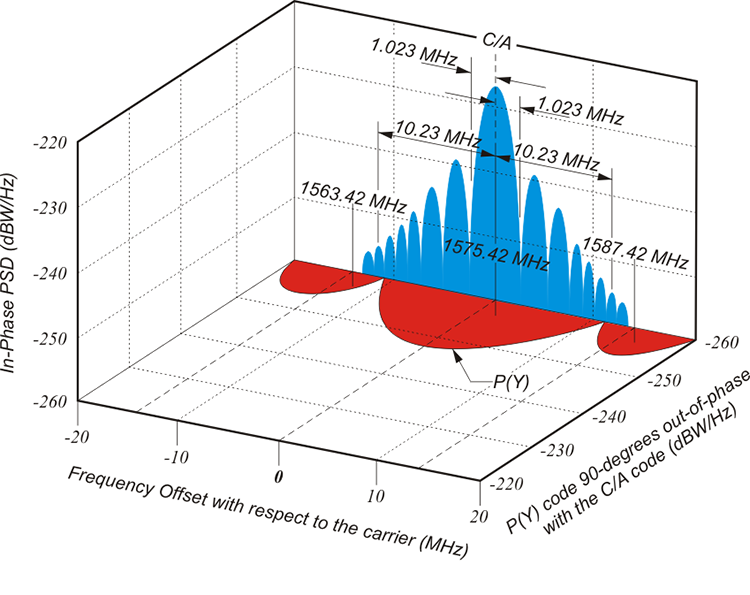
The Power Spectral Density (PSD) diagrams show the increase or decrease, in decibels, of power in Watts with respect to frequency in Hertz. It allows you to see some of the things we've already discussed. For example, this is the C/A Code in the blue on the L1 carrier, which, of course, is centered at 1,575.42 megahertz and then spread over a bandwidth that is spread spectrum. It's about 10.23 megahertz on each side for a total of like 20.46. That in the red, you see the P(Y) Code is in quadrature 90 degrees from the C/A Code. It has really one main lobe and then two sidebands, and then the blue C/A Code has many lobes.
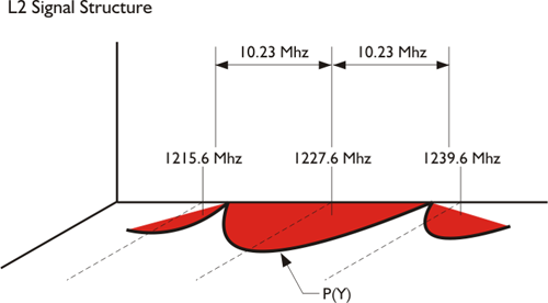
The L2 signal diagram is centered on 1,227.60 MHz. As you can see, it is similar to the L1 diagram except for the absence of the C/A code which is, of course, not carried on the L2 frequency. As well-known as these are, this state of affairs is changing.
Power Spectral Density Diagrams
Many of the improvements in GPS are centered on the broadcast of new signals. Therefore, it is pertinent to have a convenient way to visualize all the GPS and GNSS signals that illustrate the differences in the new signals and a good deal of signal theory as well. It is a diagram of the power spectral density function (PSD). They graphically illustrate the signal's power per bandwidth in Watts per Hertz as a function of frequency. In GPS and GNSS literature, the PSD diagram is often represented with the frequency in MHz on the horizontal axis and the density, the power, represented on the perpendicular axes in decibels relative to one Hertz per Watt or dBW/Hz.
The actual definition of PSD is the Fourier transform of the autocorrelation function, but the idea behind them is to give you an idea of the power within a signal with regard to frequency. These graphics show the increase or decrease, in decibels, of power, in Watts with respect to frequency in Hertz, of the well-known signals on L1 and L2.
dBW/Hz
Perhaps a bit of background is in order to explain those units. A bel unit originated at Bell Labs to quantify power loss on telephone lines. A decibel is a tenth of a bel. A decibel, dB, is a dimensionless number. In other words, it's a ratio that can acquire dimension by being associated with measured units. A change of 1 decibel would be an increase or a decrease of 27 percent. A change of 3 decibels would be an increase or a decrease of 100 percent. Here are some of the quantities with which it is sometimes associated: seconds of time, symbolized dBs, bandwidth measured in Hertz, symbolized dBHz, and temperature measured in Kelvins, symbolized dBK. Since signal power is of interest here, dB will be described with respect to 1Watt, the symbol used is dBW.
dBW is a short, concise number that can conveniently express the wide variation in GPS signal power levels. dBW can represent quite large and quite small amounts of power more handily than other notations. For example, consider a value of interest in GPS signals. The value is very small, one tenth of a millionth billionth of a watt. Expressing it as 0.0000000000000001 W is a bit exhausting. It would be more convenient expressed in dBW, a value that can be derived using the formula.
where is the power of the signal.
The expression -160 dBW is immediately useful. Here's an example. A change in 3 decibels is always an increase or a decrease of 100% in power level. Stated another way, a 3-decibel increase indicates a doubling of signal strength and a 3-decibel decrease indicates a halving of signal strength. Therefore, it is easy to see that a signal of -163 dBW has half the power of a signal of -160dBW. Considering the broadcasts from the current constellation of satellites, the minimum power received from the P code on L1 by a GPS receiver on the Earth's surface is about -163 dBW, and the minimum power received from the C/A code on L1 is about -160dBW. This difference between the two received signals is not surprising, since at the start of their trip to Earth they are transmitted by the satellite at power levels that are also 3 decibels apart. The P code on L1is transmitted at a nominal +23.8 dBW (240 W), whereas the nominal transmitted power of the C/A code on L1 is +26.8 dBW (479 W). It is interesting to note that the minimum received power of the P code on L2 is even less at -166 dBW, and its nominal transmitted power is +19.7 dBW (93 W).
One might wonder why there are such differences between the power of the transmitted GPS signal, called the Effective Isotropic Radiated Power (EIRP), and the power of the received signal. The difference is large. It is 186 to 187 dB, nearly 10 quintillion decibels. The loss is mostly because is the 20,000 km distance from the satellite to a GPS receiver on the Earth. There is also an atmospheric loss and a polarization mismatch loss, but the biggest loss by far, about 184 dB, is along the path in free space.
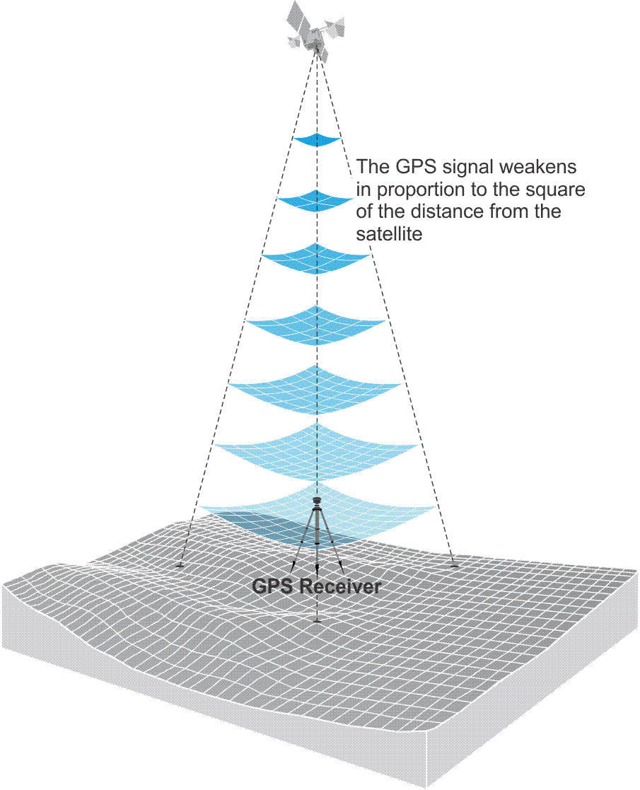
Much of this loss is a function of the spreading out of the GPS signal in space, as described by the inverse square law. The intensity of the GPS signal varies inversely to the square of the distance from the satellite. In other words, by the time the signal makes that trip and reaches the GPS receiver, it is pretty weak, as shown in the 'Inverse Square Law' figure above (Figure 8.3 from the textbook). It follows that GPS signals are easily degraded by vegetation canopy, urban canyons, and other interference.
A GPS signal has power, of course, but it also has bandwidth. PSD is a measure of how much power a modulated carrier contains within a specified bandwidth. That value can be calculated using the following formula and allowing that there is an even distribution of 10-16 W over the 2.046 MHz C/A bandwidth of the C/A code:
The calculation is also frequently normalized and done presuming an even distribution of 1W over the 2.046 MHz C/A bandwidth of the C/A code. In other words, the following calculation presumes an even distribution of the power over 1W instead of the 10-16 W used in the previous calculation: