Review:
Optical Resolution = 0.5λ/NA
Spatial Sampling = FOV/1024
Effect of changing optical resolution and spatial sampling
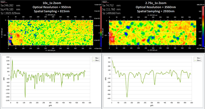
Below is an example of the effect of optical resolution and spatial sampling on information calculated from the surface data. It compares data collected with a 2.75X (NA = 0.08, FOV = 3.00 mm) objective with that from a 10X (NA = 0.3, FOV = 0.83 mm) objective. Since both the NA and the FOV change, our optical resolution and spatial sampling change. The 10X objective is able to capture finer details, and we see the surface roughness increase.
- Sa = surface arithmetic average roughness
- Sq = surface RMS roughness
- Sz = Peak to Valley difference
Effect of changing spatial sampling while using the same optical resolution
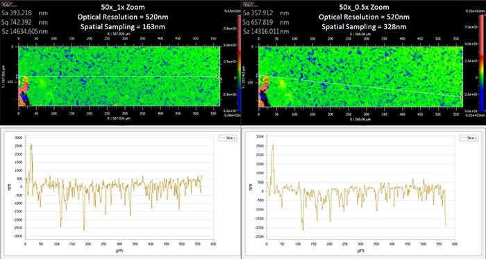
In the below example, the optical resolution is kept the same, both are using the 50X objective (NA = 0.55). However, we are using the internal magnification (0.5X, 1.0X, 2.0X) to change the FOV, which affects the spatial sampling. Even though it has the same resolution, the results collected are affected by the different spatial sampling.
- Sa = surface arithmetic average roughness
- Sq = surface RMS roughness
- Sz = Peak to Valley difference
Note
Be very careful when comparing data from different scans. The above examples illustrate that numerical values from surfaces should only be compared if they were collected using the same optical resolution and spatial sampling.