11.3 The Story of Diurnal Boundary Layer Growth Told in Vertical Profiles of Virtual Potential Temperature
Recall the concept of virtual potential temperature, which was introduced in Lesson 2. The virtual potential temperature is found by replacing the temperature in the formula for virtual temperature with the potential temperature:
θv is the virtual potential temperature. It is a useful quantity because it takes the moisture into account as well as temperature when considering buoyancy and stability. Thus, adiabatic ascent or descent in moist air follows the constant virtual potential temperature line all the way up to the lifting condensation level (LCL), where the potential temperature increases. So let’s look at the evolution of the profile of virtual potential temperature in a cloud-free boundary layer.
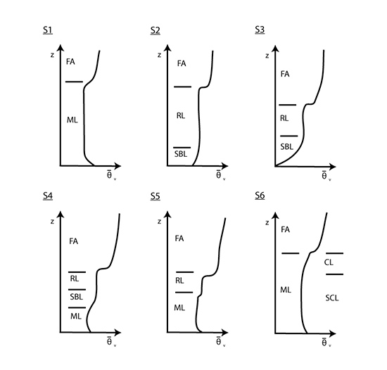
Start with the late afternoon (S1 above). Surface heating causes the air near the surface to have a higher virtual potential temperature than the air just above it, so that the air is superadiabatic. Thus, air parcels of this warm moist air rise into the mixed layer, warming this layer of air. Some of the warm moist parcels (also called convective eddies) rise all the way up to the point in the free atmosphere where the virtual potential temperature is as great or greater than the air parcel’s value. At this point the air parcel likely mixes with the surrounding air. Mixing the warm free-tropospheric air into the mixed layer, which is called entrainment, also causes the daytime mixed layer to warm. Turbulent drag at Earth's surface also contributes to the turbulence in the boundary layer. The result of this vigorous convective activity is a well-mixed boundary layer.
Just after sunset (S2 above), the surface cools by infrared radiation and the air near the surface becomes thermodynamically stable with a virtual potential temperature (and thus temperature) inversion. As in the day, turbulent drag at Earth's surface creates turbulent mixing, but the air's thermodynamically stability suppresses this vertical mixing. As a result, the nocturnal boundary layer on a calm night becomes quite stable, and, as the surface continues to cool, the boundary layer becomes even more stable during the night (S3 above). On a windy night, the nocturnal layer is closer to well-mixed, but only if the turbulent drag is strong enough to counter the infrared radiative cooling at Earth's surface. The stable boundary layer grows, not by convective mixing, but by turbulent drag at Earth's surface and sometimes by shear-drive mixing at the top of this layer.
Just after sunrise (S4 above), the surface is warmed by the sun, and as it continues to get warmed throughout the morning (S5 above), convection begins to mix warm air up first throughout the stable boundary layer and then into the mixed layer. Any trace atmospheric constituents left in the residual layer from the day before are now mixed back into the boundary layer as it grows higher. Finally, the residual layer is entirely mixed into the growing boundary layer, and the boundary layer returns to its condition of the previous afternoon (S1 above). If conditions are right, a convective cloud layer may form at the top of the mixed layer (S6 above).
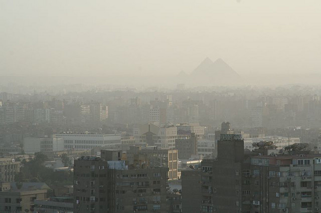
Think about morning and evening rush hours. During morning rush hour, which is near sunrise, the vehicle emissions mix into a shallow boundary layer and hence the mixing ratios of the pollutants can be quite substantial. This situation leads to the photochemistry that makes pollution, including ozone. In the evening, the rush hour traffic also emits the same amounts of pollutants into the boundary layer, but because the boundary layer height is so much greater in the early evening than in the morning, the pollutant mixing ratios are less because the same level of emissions are being mixed into a larger volume of air. Thus the effects of evening emissions are not as severe as the effects of morning emissions. In addition, modeling the planetary boundary layer height correctly is essential for accurate air quality modeling.
Also think about the development of convective storms. Summertime thunderstorms are most common in the afternoon and evening because many of these storms are initiated by the convective eddies in the daytime mixed layer. As the mixed layer grows, the turbulence can reach the lifting condensation level, which the level at which clouds form (see Lesson 3) and, under the right conditions, the level of free convection (again, see Lesson 3), which is the level at which convective storms begin to grow. The growth of the boundary layer is thus closely connected to the initiation of convective storms.
The diurnal variation of the planetary boundary layer height is more than just a curiosity--it has influence on our daily lives and health because we live, work, and breathe mostly in the atmospheric planetary boundary layer. Thus it is important that meteorologists and atmospheric scientists gain a better understanding of the atmospheric motions and energy budget of the planetary boundary layer. Gaining this understanding means learning something about atmospheric turbulence, which is the small-scale chaotic winds created by the interactions of the planetary boundary layer with Earth's surface.