Prioritize...
After completing this section, you should be able to describe the difference between a grid-point model and a spectral model. This description should include advantages and disadvantages of each type.
Read...
Worldwide, there are many different computer models run on a day-to-day basis that provide guidance for weather forecasters. Computer models are extremely complex, and those who design them must make decisions about how to handle many complicated mathematical problems.That means there's more than one approach to creating a numerical weather prediction model. Indeed, various models differ in their geographical area, initialization technique, representation of topography, mathematical formulation, length of forecast (in other words, how far into the future they are run), and other factors. In this section, we'll cover some basic types of computer models, along with their pros and cons. Indeed, each type has both pros and cons; no matter what benefits come with a particular approach, each has its own drawbacks.
For starters, models differ in the geographic area that they cover, which is called the model domain. Some models cover the entire Earth (they have a "global domain"), and are therefore often called "global models." Some of the most rigorously developed and commonly used global models are the:
- Global Forecast System (GFS) model (run by the National Centers for Environmental Prediction in the United States)
- ECMWF (run by the European Centre for Medium-Range Weather Forecasts -- sometimes called "the Euro")
- CMC GDPS (Global Deterministic Prediction System run by the Canadian Meteorological Centre -- sometimes called "the Canadian model")
- UKMET (run by the UK Met Office).
However, other nations, such as Germany, France, Japan, and India also run global weather prediction models. Forecast data from many of these models are publicly available on the web for free, although some models like the ECMWF only offer a limited suite of free forecast data (the complete set of forecast data is only available to paying customers).
Other models have more limited domains and only cover specific regions of the globe. One such commonly used model is the North American Mesoscale model (NAM; pronounced "nam" -- rhymes with "jam"). As you probably guessed from the name, the NAM focuses on North America and its immediate surroundings. Regional models can only produce forecasts for locations within their domain, which is clearly a limitation. The main benefit of regional models is that they can often produce more "detailed" forecasts than global models can. To get a better idea of what I mean by "detailed," let's investigate "grid-point models" and "model resolution."
Grid-Point Models
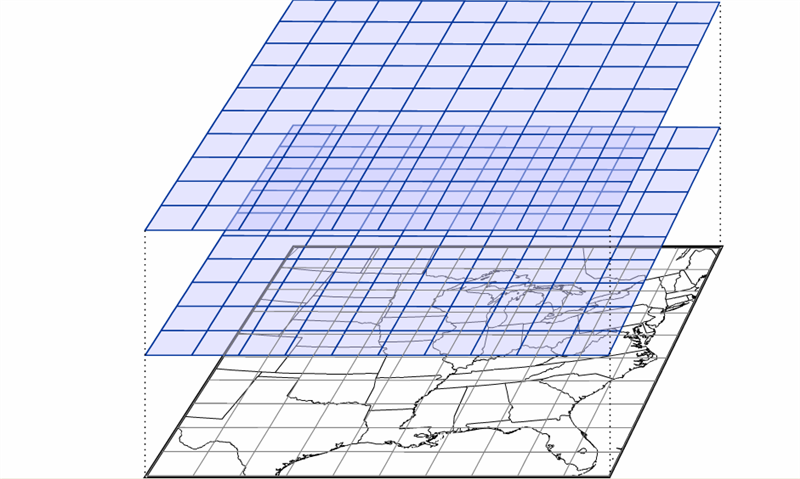
Many weather models, such as the NAM, are referred to as a grid-point models because the mathematical equations are calculated on a grid in three dimensions (see image below). The spacing of the grid is referred to the model resolution, and usually, the larger the model domain, the coarser the resolution (larger grid spacing). So, regional models like the NAM are often capable of higher resolutions (less space between the grid points where the model performs calculations), which allows for more detailed forecasts. That's definitely an advantage for regional models!
Over the years, the NAM model has operated using various calculation schemes -- the "guts" of the model. Currently, the model uses a scheme called NEMS-NMMB (short for: NOAA Environmental Modeling System - Non-hydrostatic Multi-scale Model), which allows for multiple domains and resolutions to be run simultaneously. Note the various resolutions of the different NAM domains. Some of the NAM's domains have resolutions of just a few kilometers, which can generate very detailed forecast simulations.
But, even grid-point models that can create detailed forecast simulations have a problem. To see what I mean, check out the image below, which shows a type of map commonly used by weather forecasters to assess weather patterns above the Earth's surface. Forecasters often look at analyses showing the height at which the atmospheric pressure is a specific value (a pressure of 500 millibars is one common pressure level, which is about half of typical pressure values at sea level), and this is a polar stereographic perspective of the 500-mb height pattern for March 1, 2012. This perspective allows you to easily see the numerous waves positioned around the globe. Now, compare to this "gridded" version of this height data. It looks a lot different, doesn't it? We've largely lost the sense of the waves that make up the 500-mb pattern, and some of the finer features have vanished. In reality, most atmospheric variables aren't really well represented by "boxes." Grid-point models with high resolutions have smaller "boxes", but they still can't perfectly simulate the real atmosphere, even though they employ sophisticated interpolation schemes to smooth out the data.
Model developers have come up with some sophisticated techniques for reducing the "box-like" nature of model grids, so not all grid-point models use square or rectangular grids to perform their calculations about future states of the atmosphere. Indeed, some models employ grids that look more like hexagons (credit: NCAR), and some models have flexible grids, which allow for different grid sizes over different parts of the globe (credit: NOAA) in order to "zoom in" and give more detailed predictions in and around important weather features. The grid style that a particular model employs can have consequences for calculation efficiency and accuracy, so model developers often have to balance computational speed and forecast accuracy when deciding what type of grid to use (each has pros and cons).
Spectral Models
Still, many variables in the atmosphere, like the 500-mb heights you saw above, are better represented by wave-like structures than any type of grid, and it turns out there's another type of model, called a spectral model, that isn't based on grids. Rather than dividing up the atmosphere into a series of grid boxes, spectral models describe the present and future states of the atmosphere by solving mathematical equations whose graphical solutions consist of a series of waves. I'll skip the details of the mathematics since they're outside the scope of this class, but the key concept lies in the idea that any wave-like function can be replicated by adding various simple waves together. As an example, check out the figure below. Consider a 500-mb height pattern that follows the green line. A spectral model first approximates this pattern by adding a series of simple wave functions, described mathematically by the function called "sine." In our example, I was able to closely duplicate the green curve by adding together three different wave functions (the red, blue, and purple curves). The resulting black curve is fairly close to the green curve and has a simple (relatively speaking) equation that the computer has no problem interpreting.
Spectral models thus begin by first analyzing current patterns in the observed atmospheric variables and then recreating those patterns using sums of simple wave functions. The advantage of a spectral model is that the way in which the sine function changes is well known, and we don't need a set of gridded observations at all!
The fact that we know exactly how a wave function will change in time and space brings us to the major advantage of spectral models: They save computational time, and that can be a big advantage when a model is producing longer-range forecasts. But, spectral models have shortcomings, too. First, spectral models don't perform well on regional domains (domains with fixed boundaries) because the sine functions that make up the "waves" in the model are unbounded. They don't artificially end at the boundary of some arbitrary regional domain. The waves extend all the way around the earth, reconnecting where they began; therefore, most spectral models are global models (although some global models are grid-point models).
Another shortcoming of spectral models is that while many atmospheric variables exhibit a wave-like appearance (the 500-mb height pattern, for example), some most definitely do not. Think about a day with spotty showers and thunderstorms. The spatial pattern of precipitation in this case certainly does not lend itself to smooth, wave-like functions. The same goes for any variable with an abrupt gradient or discontinuity. For predicting such variables, spectral models just aren't ideal. Model developers try to overcome such obstacles by incorporating internal grids to calculate troublesome variables and feed them back into the spectral mathematics. It's a rather complex and imperfect process, but it's part of the never-ending process of trying to limit model shortcomings.
Finally, I should point out that spectral models are not immune from computational error. It turns out that a finite sum of wave functions cannot exactly reproduce every wave pattern. Notice the subtle differences between the black and green curves in the figure above. These differences arise because I am only adding together three different wave patterns. If I were to increase that number to 10 or 20 different waves, the match would be much closer (but still not perfect). Spectral models measure their "resolution" in the number of waves that can be added together to reproduce a particular pattern. At some point, you have to stop adding in new functions and the difference between the actual pattern and the pattern that you reproduced is called truncation error. As in the figure above, our approximation of the observed pattern may be very good, but it takes only a very small amount of error to start leading the model astray. There's also the ever-persistent problems of observational error and round-off error to contend with as well (not to mention the computational error from the grid-point part of the model). Thinking about all of the sources of error makes you wonder how computer models predict the weather as well as they do!
Now that you understand some of the basics behind numerical weather prediction, let's get down to actually retrieving model data from the rNOMADS server.
Read on.