Prioritize...
At this point, you should be familiar with retrieving model analysis data from the NOMADS server. In this section, we will look at how to retrieve various numerical forecast data from the server as well. Make sure you spend time experimenting with the code below, as this is the only way of becoming comfortable with using the R-code. When you are ready, complete the Quiz Yourself challenge.
Read...
Of course, the reason why we are interested in retrieving model data in the first place is to get a suggestion of what the future might hold. As always, use numerical predictions with caution, especially at forecast times beyond 48-hours. Over the course of this program, you will learn the proper treatment of computer model data, but, for now, let's just see what kinds of data we can retrieve from the NOMADS server.
Remember that computer models gather all sorts of observations that are used to form the initial state or model analysis. At that point, the model equations are "run" forward in time, and forecasts for numerous variables are generated at prescribed intervals in the future. You might imagine the possibilities for analysis... The GFS model contains 251 variables (some at multiple levels) predicted for over 250K points at 80 different forecast times! This is a massive amount of data, but, fortunately, R can do the heavy lifting.
Let's start with a simple form of the code from the previous page. Since we know what we are looking for, we can skip a few steps...
# check to see if rNOMADS has been installed
# if not, install it
if (!require("rNOMADS")) {
  install.packages("rNOMADS") }

library(rNOMADS)

#get the latest GFS 0.5x0.5 model url
latest.model <- tail(GetDODSDates("gfs_0p50")$url, 1)

# Get the latest model run for this date
latest.model.run <- tail(GetDODSModelRuns(latest.model)$model.run, 1)

variable <- "tmp2m"  # 2-meter temperatures
time <- c(0, 80)     # Get all 80 forecast times
lon <- c(560, 580)   # Get only a small subset of points
lat <- c(260, 270)   #   around my location of interest
lev<-NULL            # DO NOT include level if variable is non-level type

model.data <- DODSGrab(latest.model, latest.model.run,
                       variable, time, levels=lev, lon, lat)
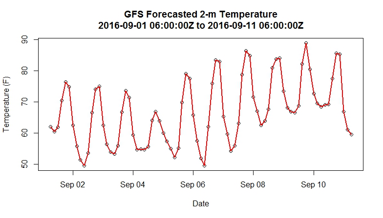
Notice that the main difference in this script is that we are asking the server for all of the model forecasts (for this model, there are 8 forecasts per day for 10 days). What we are after is a time series of forecast 2-meter temperatures at one particular grid point (the nearest grid point to State College, PA). After retrieving the data, we simply need to clean it up a bit and plot it using the following code.
# Switch the lat/lon coordinate system around
model.data$lon<-ifelse(model.data$lon>180,model.data$lon-360,model.data$lon)

# Get two vectors one temperature and one dates/times
# at only a single grid point
model.temperature<-model.data$value[which(model.data$lon==-78 & model.data$lat==41)]
model.fdate<-model.data$forecast.date[which(model.data$lon==-78 & model.data$lat==41)]

# Convert to Fahrenheit
model.temperature<-(model.temperature-273.15)*9/5+32

# Display times in GMT
attr(model.fdate, "tzone") <- "GMT"

# Make a plot
plot(model.fdate,model.temperature,
     xlab = "Date", ylab = "Temperature (F)",
     main = paste0("GFS Forecasted 2-m Temperature\n",
                  head(model.fdate,1),"Z to ",tail(model.fdate,1),"Z")
     )
lines(model.fdate,model.temperature,lwd=2,lty=1,col="red")
Your plot of forecast 2-m temperatures should resemble the one below. You might see if you can figure out how to alter the entire script to select a point of your choosing. For more flexibility, you could retrieve a larger set of points (the entire U.S., for example) but bear in mind that you are retrieving 80 grids (one for each forecast time) worth of data. So, your retrieved file will grow substantially if your requested domain is large.
Quiz Yourself...
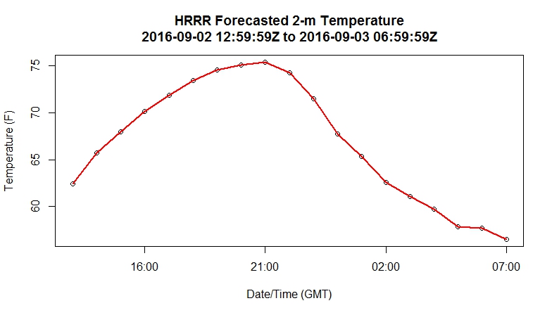
The HRRR (model code: "hrrr") is a very high-resolution, short-term model centered over the continental U.S (check out this sample 2-m temperature plot from the HRRR). Instead of producing output four times a day, the HRRR creates a forecast for each hour. Can you alter the code above to retrieve the 2-meter temperature for the meteorology building at Penn State (40.793313 N, 77.866796 W) or any other point of your choosing? I have hidden my script, but show you the resulting plot below.
My solution:
You may have approached the problem in an entirely different manner (and that's fine). However, I wanted to point out a few extra changes I made to the code. First, I used the extract_info function that I introduced in the "Explore Further" section on the previous page. It's not necessary that you do so; you could have simply copied down the model parameters from the model.run.info file. Since I already had the function, I reused it. This is an important lesson to remember... if you write good scripts with plenty of commenting, you can likely reuse/adapt them for future projects. Being organized when it comes to creating scripts will pay off, believe me.
Next, since the HRRR model resolution is not 0.5 degrees like the GFS, it can be quite a pain to figure out what model points in order to capture my location of interest within the smallest box possible. You certainly don't want to retrieve them all (the HRRR has many thousands more points than the GFS). Therefore, I created the formulas to solve for the number of points needed, given a longitude/latitude and the model resolution. I discovered in this process that the model resolution given in model.run.info was not the actual resolution but instead a rounded value (why, I have no idea). This caused problems, and thus I needed to figure out the actual resolution by doing a test retrieval first, figuring out the step-size in lat/lon, and then entering those values in my formula. It occurred to me that it might have been easier and quicker just to guess the number of points necessary, but in the end, I now have something that works for any point I choose.
Finally, after I retrieved the model data, I needed to figure out what grid point was closest to my chosen location. This process is easy for the GFS because I know that the points fall every half of a degree (70.0, 70.5, 71.0, etc). With the HRRR, the task is a bit more complicated. Therefore, I use a pseudo-distance test to determine the best grid point being the one that is less than half the model resolution in each direction.
# check to see if rNOMADS has been installed
# if not, install it
if (!require("rNOMADS")) {
  install.packages("rNOMADS") }

library(rNOMADS)

extract_info <- function(x) {
  lonW<-as.numeric(as.character(sub("^.*: (-?\\d+\\.\\d+).*$","\\1", x[3])))
  lonE<-as.numeric(as.character(sub("^.*to (-?\\d+\\.\\d+).*$","\\1",x[3])))
  lonPoints<-as.numeric(as.character(sub("^.*\\((\\d+) points.*$","\\1", x[3])))
  lonRes<-as.numeric(as.character(sub("^.*res\\. (\\d+\\.\\d+).*$","\\1", x[3] )))
  latS<-as.numeric(as.character(sub("^.*: (-?\\d+\\.\\d+).*$","\\1", x[4])))
  latN<-as.numeric(as.character(sub("^.*to (-?\\d+\\.\\d+).*$","\\1",x[4])))
  latPoints<-as.numeric(as.character(sub("^.*\\((\\d+) points.*$","\\1", x[4])))
  latRes<-as.numeric(as.character(sub("^.*res\\. (\\d+\\.\\d+).*$","\\1", x[4] )))
  out<-data.frame(lonW,lonE,lonPoints,lonRes,latN,latS,latPoints,latRes)
  return (out)
}

#get the latest HRRR model url
latest.model <- tail(GetDODSDates("hrrr")$url, 1)

# Get the latest model run for this date
latest.model.run <- head(GetDODSModelRuns(latest.model)$model.run, 1)

# Get info for a particular model run
model.run.info <- GetDODSModelRunInfo(latest.model, latest.model.run)
model.domain<-extract_info(model.run.info)

# Here's the point I want
my_lat <- 40.793313
my_lon <- -77.866796

# I used a formula to calculate what points I should retrieve
variable <- "tmp2m"  # 2-meter temperatures
time <- c(0, 18)     # Get all 80 forecast times
lon <- c(floor((floor(my_lon)-model.domain$lonW)/0.029240189), floor((ceiling(my_lon)-model.domain$lonW)/0.029240189))
lat <- c(floor((floor(my_lat)-model.domain$latS)/0.027272727), floor((ceiling(my_lat)-model.domain$latS)/0.027272727))
lev<-NULL            # DO NOT include level if variable is non-level type

model.data <- DODSGrab(latest.model, latest.model.run,
                       variable, time, levels=lev, lon, lat)

# Get two vectors one temperature and one dates/times
# at only a single grid point
model.temperature<-model.data$value[which(abs(my_lon-model.data$lon) < model.domain$lonRes/2 & abs(my_lat-model.data$lat) < model.domain$latRes/2)]
model.fdate<-model.data$forecast.date[which(abs(my_lon-model.data$lon) < model.domain$lonRes/2 & abs(my_lat-model.data$lat) < model.domain$latRes/2)]

# Convert to Fahrenheit
model.temperature<-(model.temperature-273.15)*9/5+32

# Display times in GMT
attr(model.fdate, "tzone") <- "GMT"

# Make a plot
plot(model.fdate,model.temperature,
     xlab = "Date/Time (GMT)", ylab = "Temperature (F)",
     main = paste0("HRRR Forecasted 2-m Temperature\n",
                   head(model.fdate,1),"Z to ",
                   tail(model.fdate,1),"Z")
)
lines(model.fdate,model.temperature,lwd=2,lty=1,col="red")
Did your graph resemble mine?