Prioritize...
We have retrieved model data in the horizontal plane and in time. In this section, we will look at retrieving profiles of model data. As always, make sure that you follow along with your own version of the code. After you get this sample working, experiment with variations so that you are comfortable with the commands.
Read...
So far, we have examined how to access model data both in horizontal space and in time. Before moving on to other forms of model data, I wanted to demonstrate an example of extracting model data in the vertical dimension.
Computer models have several different vertical coordinate systems. At lower levels, there are many variables defined at specific heights above the ground (2-meter temperature is an example). There are also a group of variables that are defined over an array of pressure levels (called the mandatory levels). These variables are defined by both lat/lon coordinates and a height coordinate. Let's see how we can retrieve them from a model file.
We start with the standard query of the NOMADS dataset...
# check to see if rnoaa has been installed
# if not, install it
if (!require("rNOMADS")) {
  install.packages("rNOMADS") }

library(rNOMADS)
library(reshape2)

#get the available dates and urls for this model (14 day archive)
model.urls <- GetDODSDates("gfs_0p50")

latest.model <- tail(model.urls$url, 1)

# Get the model runs for a date
model.runs <- GetDODSModelRuns(latest.model)

latest.model.run <- tail(model.runs$model.run, 1)

# Get info for a particular model run
model.run.info <- GetDODSModelRunInfo(latest.model, latest.model.run)

# variables that are pressure level dependent...
# model.run.info[grep("1000 975", model.run.info)]
If you want to identify what variables are defined at the mandatory levels, you can query model.run.info using the command directly above. Notice below that I am retrieving three variables in one call. I am also limiting my lat/lon box to save space, and I am requesting all 46 levels.
# I'm retrieving temperature, RH, and geopotential height
variable <- c("tmpprs","rhprs","hgtprs")
time <- c(0, 0) #Analysis run, index starts at 0
lon <- c(560, 580)
lat <- c(260, 270)
lev<-c(0,46)  # Requesting level-type variables, so we can use this parameter

model.data <- DODSGrab(latest.model, latest.model.run, variable, time, levels=lev, lon, lat)
model.data$lon<-ifelse(model.data$lon>180,model.data$lon-360,model.data$lon)

# Get the lat/lon point I want (41N, 78W)
# I could have made this a variable
profile.data <- data.frame(
   Level=model.data$levels[which(model.data$lon==-78 & model.data$lat==41)],
   Vars=model.data$variables[which(model.data$lon==-78 & model.data$lat==41)],
   Values=model.data$value[which(model.data$lon==-78 & model.data$lat==41)]
)

# reshape the output into proper columns
profile.dcast <- dcast(profile.data, Level~Vars)

# add a column of converted temperature
profile.dcast <-transform(profile.dcast, TempC=(tmpprs-273.15))
Now, let's plot the results. Notice that I used my mfrow command again so that I can plot two graphs side-by-side.
# multiple plots... 1 row, 2 columns
# we also do some margin and graph size control here
par(mfrow=c(1,2), oma=c(0,1,2,1)+0.1, mar=c(0,0,3,0), pin=c(3.4,5))

# make the first plot...
# Note that I am plotting only a subset of points
# I do this so that the two graphs can have different y-axes
# with the same range.

plot(profile.dcast$TempC[which(profile.dcast$Level>49)],
     profile.dcast$Level[which(profile.dcast$Level>49)],
     type="n", xlab = "Temperature (C)",
     ylab = "Log P (mb)", log="y", ylim = c(1000,50),
     main="Temperature")
lines(profile.dcast$TempC,profile.dcast$Level,lwd=2,lty=1,col="#CC0000")
points(profile.dcast$TempC,profile.dcast$Level,pch=19,col="#CC0000")

# make the second plot...
plot(profile.dcast$rhprs[which(profile.dcast$Level>49)],
     profile.dcast$hgtprs[which(profile.dcast$Level>49)],
     type="n", xlab = "Relative Humidity (%)", ylab = "Height (m)",
     main="Relative Humidity")
lines(profile.dcast$rhprs,profile.dcast$hgtprs,lwd=2,lty=1,col="#009900")
points(profile.dcast$rhprs,profile.dcast$hgtprs,pch=19,col="#009900")

# overall title...
title(paste0("GFS Model Profile from (41N, 78W) at ",
      format(head(model.data$forecast.date,1), "%m-%d-%Y %HZ", tz="GMT")),
      outer=TRUE, cex.main=1.6)
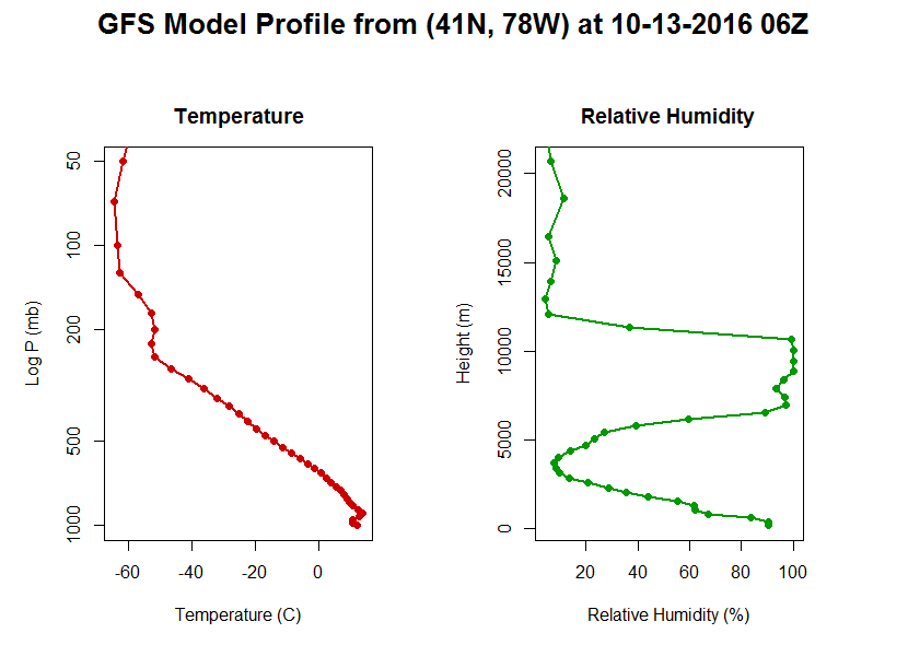
Here's my plot. Yours should look similar although the data itself will likely be different.