Moving Average Model Overview

Read...

So, we saw how we can use the periodicity of a variable for prediction through AR modeling. But, sometimes, that is not enough. Instead, it might be more beneficial to model the data based on the errors of the previous forecast. This is where a Moving Average (MA) model comes in.

General Description

The basic idea of an MA model is that the variable depends linearly on the past errors of forecasts. An MA model creates a forecast at time t and computes the forecast errors, then the model forecasts the next time stamp (t+1) using the errors computed from the previous forecast (time t) as predictors. In short, the moving average model is the weighted average of past errors. Mathematically, an MA model looks like:

where μ is the mean of Y_t+1, $\epsilon$ are the forecast errors for the current forecast (time t) and the previous (t-1) and $\beta$ are the parameters of the model. Similar to the AR model, the MA model has an order saying how many past errors to include, denoted by MA(q). The above equation is an example of an MA model of order 1, MA(1). An MA(2) is given by the following equation:

And the qth order is:

There are some basic requirements for an MA model. For one, the time series is assumed to be stationary. The errors are assumed to be independently normally distributed. You can see this equation looks very similar to the AR model. So what is the main difference? A pure AR model depends on the lagged values of the data while a pure MA model depends on the previous forecast errors.

Advantages and Disadvantages

The MA model is great because it’s computationally efficient and yields a very stable forecast, in that it doesn’t change drastically from one value to another. In addition, an MA model can be updated every time a new forecast is made; that is, you add in the forecast errors and update the model.

There are, however, several disadvantages. For one, an MA model requires you to save past forecast errors to create a new model and predict the next value. This is costly in terms of computational memory. The MA model also ignores complex relationships; it is focused on characterizing the mean value instead of capturing the natural fluctuations that occur. This, in turn, can remove extreme values as the MA model focuses on the average. 

How to tell if an MA model is a good fit?

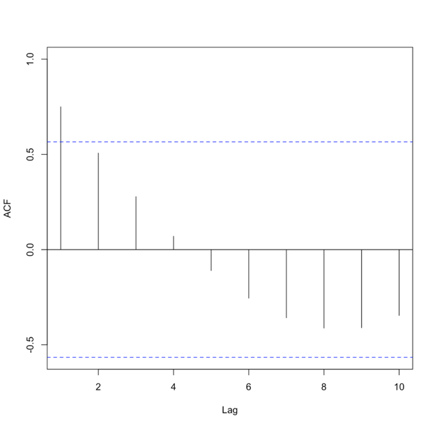
Similar to the AR model, we look to the autocorrelation for insight. In this case, we will examine the ACF. We use an MA(1) when there is only a significant autocorrelation at lag 1. For example:

Example of ACF for an MA(1) model

Credit: J. Roman

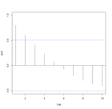
When there are significant correlations at lags 1 and 2 but no significant correlations at higher lags, we use an MA(2). The ACF would look like this:

Example of ACF for an MA(2) model

Credit: J. Roman

You should start to see the pattern. An MA(q) model would be selected when there are significant autocorrelation values for the first q lags and nonsignificant autocorrelation for lags>q. So, what’s the key difference between the AR and MA in terms of the ACF. An AR model will have an ACF that exponentially decreases to 0 as the lag increases, where an MA model will have an ACF that has significant correlations for the first q lags and then autocorrelation=0 (or nonsignificant) for all lags >q. For a PACF, in an AR model, the number of non-zero partial autocorrelation provides the order for the AR model (the most extreme lag of the variable that is used for prediction). Whereas, in an MA model, the PACF tapers toward 0. For the AR model, we tend to use the PACF, while for the MA model, we will use the ACF. 

Let's try and create an MA model in R using our precipitation data from Bangkok. We start by creating the ACF. Use the code below:

# create acf of data
precipACF <- acf(monthlyPrecip)

You should get the following figure:

ACF for monthly precipitation in Bangkok, Thailand

Credit: J. Roman

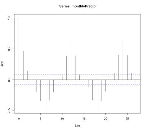
Like I said above, an MA model has an ACF with the characteristic that the correlation will be strong for q lags and then become nonsignificant. This is not a good candidate for MA modeling! However, we will test out an MA model to see how well It does compare to the AR model.

For the MA model, we will use the function ‘auto.arima’. I will not talk a lot about this function right now because we will use it in the following sections. For now, to create a pure MA model, we will set the following parameters: d=0, D=0, max.p=0, max.P=0, max.d=0, max.D=0. These parameters will be discussed in more detail later on. Use the code below to create an MA model. The ‘auto.arima’ function selects the best model by using either the AIC, AICC, or BIC metric.

# create MA model 
precip_MA <- auto.arima(monthlyPrecip[1:(length(monthlyPrecip)-100)],ic="aic",d=0, D=0, max.p=0, max.P=0, max.d=0, max.D=0)

For this example, the best MA model was of order 2 (simply type out precip_MA and the information will pop up). If we use the summary function, we can obtain a number of error measures from the training data, including the RMSE which in this case was 4.5 inches, close to the AR(1) model.

Unlike the AR model, predicting data is not as simple as before because with the MA model, we update based on the errors of the previous forecast. So for each prediction, we need to update the MA model. Use the code below to forecast the last 100 points of precipitation.

# predict values 
precipMA_predict<-{} 
for(i in 1:100){ 
  dataSubset <- monthlyPrecip[(i:(length(monthlyPrecip)-101+i))] 
  precip_MA=auto.arima(dataSubset,ic="aic",d=0, D=0, max.p=0, max.P=0, max.d=0, max.D=0) 
  precipMA_predict[i] <- predict(precip_MA,n.ahead = 1)$pred 
}

Now, plot the predicted vs the observed.

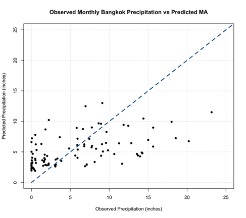
# predict values 
dataObserved <- monthlyPrecip[(length(monthlyPrecip)-99):length(monthlyPrecip)] 
plot.new() 
grid(nx=NULL,ny=NULL,'grey') 
par(new=TRUE) 
plot(dataObserved,precipMA_predict,xlab="Observed Precipitation (inches)", 
     ylab="Predicted Precipitation (inches)",main="Observed Monthly Bangkok Precipitation vs Predicted MA", 
     xlim=c(0,25),ylim=c(0,25),pch=16) par(new=TRUE) plot(seq(0,30,1),seq(0,30,1),type='l',lty=2,col='dodgerblue4',lwd=3,xlab="Observed Precipitation (inches)", 
     ylab="Predicted Precipitation (inches)",main="Observed Monthly Bangkok Precipitation vs Predicted MA",   
     xlim=c(0,25),ylim=c(0,25))

You should get the following figure:

Predicted precipitation versus observed precipitation for Bangkok, Thailand using an MA model

Credit: J. Roman

Now, a good thing to note is with an MA model you are less likely to get unrealistic values, but we should still check. You can do this by determining the minimum value of the predictions. Note that, depending on your variable, you may need to check multiple constraints (including a maximum value).

Back to the interpretation, similar to the AR model, this MA model does not look to be the best fit. We do not see many values along the 1-1 line and paired with the error measure scores, the MA model is not the greatest at modeling the monthly Bangkok Precipitation. But that doesn’t mean the MA model is worthless in this example; it just means that neither the AR or MA are the best, and each has its own skill. So, what if we could combine the strengths of both?