Prioritize...
After reading this section, you should be able to fit an ARIMA/ARMA model to data when applicable.
Read...
We saw in our previous examples that a pure AR model did not do a great job at predicting precipitation in Bangkok. Similarly, a pure MA model fell short. But both models provide quality information, so let’s try combining them to create a better model.
ARIMA Example
Before we create the ARIMA model, we actually should look into whether ARMA or ARIMA is more appropriate; that is, does a trend or other chaotic periodicities exist in our data? We can check this by plotting the time series.
Your script should look something like this:
# plot time series
plot.new()
grid(nx=NULL, ny=NULL, 'grey')
par(new=TRUE)
plot(date[time_index],monthlyPrecip,xlab="Time",ylab="Monthly Precipitation (inches)",
     main="Bangkok, Thailand Precipitation",type="l")
You should get a figure like this:
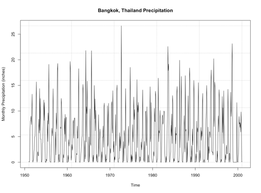
By examining this figure, there doesn’t appear to be an overall trend of increasing or decreasing precipitation. An alternative method is to look at the anomaly which tends to paint a clearer picture. Here is a time series of the anomaly, with the 0 line highlighted in blue.
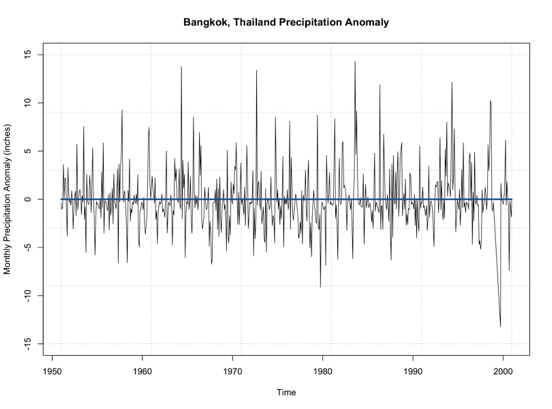
Note that the time series doesn’t really increase or decrease. It’s not drifting from the 0 line, but simply fluctuating around it. This leads me to believe that no differencing is needed for stationary as it pertains to non-periodicity. Let’s see if this is true and use the ‘auto.arima’ function. Again, this function will select the best ARIMA model with the best p,d,q parameters based on AIC scores of several models. Use the code below to create an ARIMA model.
Your script should look something like this:
# create ARIMA model
precip_ARIMA <- auto.arima(monthlyPrecip[1:(length(monthlyPrecip)-100)],ic="aic",seasonal=FALSE)
The main difference from our previous MA example is I let the function choose the p,d, and q values as opposed to the pure MA where I set p and d to 0 to ensure a pure MA model was selected. Ignore the seasonal parameter for now; we will discuss this in more detail later on. When I run this, the model selected is ARIMA(5,0,1) which can be called ARMA(5,1). So, like we saw in the plot, the ARIMA model selected d=0; differencing is not needed due to trends in the data.
We can look at the summary metrics again (using summary()). The RMSE is 4.1 inches. You can also compare how the model predicted the training dataset observations. Remember, this is not the best approach because the model is using these observations. But let’s give it a try.
Your script should look something like this:
# plot Training Data vs Predictions
plot.new()
grid(nx=NULL,ny=NULL,'grey')
par(new=TRUE)
plot(precip_ARIMA$x,precip_ARIMA$fitted,xlab="Observed Precipitation (inches)",
     ylab="Predicted Precipitation (inches)",main="Observed Monthly Bangkok Precipitation vs Predicted ARMA",
     xlim=c(0,25),ylim=c(0,25),pch=16)
par(new=TRUE)
plot(seq(0,30,1),seq(0,30,1),type='l',lty=2,col='dodgerblue4',lwd=3,xlab="Observed Precipitation (inches)",
     ylab="Predicted Precipitation (inches)",main="Observed Monthly Bangkok Precipitation vs Predicted ARMA",
     xlim=c(0,25),ylim=c(0,25))
You should get this figure:
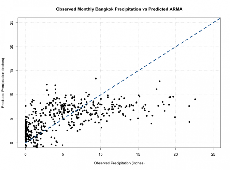
One of the things that hopefully popped out was the negative values once again. We must consider the constraints of the data and realize that our models don’t necessarily ‘know’ those constraints, so we must impose them ourselves.
One of the great things about ARMA/ARIMA is the opportunity to update the model regularly. And in reality, we probably would update the model with new observations to adjust it ever closer to reality. So let’s go ahead and set up an algorithm that forecasts the monthly precipitation one month out using the most relevant observations to create a model. Then, we can plot the observations vs the predictions.
Your script should look something like this:
# predict values
precipARIMA_predict<-{}
for(i in 1:100){
  dataSubset <- monthlyPrecip[(i:(length(monthlyPrecip)-101+i))]
  precip_ARIMA=auto.arima(dataSubset,ic="aic",seasonal=FALSE)
  precipARIMA_predict[i] <- predict(precip_ARIMA,n.ahead=1)$pred
}
And now, let’s plot.
Your script should look something like this:
# plot predicted and observed values
dataObserved <- monthlyPrecip[(length(monthlyPrecip)-99):length(monthlyPrecip)]
precipARIMA_predict[which(precipARIMA_predict <0)] <- NA
plot.new()
grid(nx=NULL,ny=NULL,'grey')
par(new=TRUE)
plot(dataObserved,precipARIMA_predict,xlab="Observed Precipitation (inches)",
     ylab="Predicted Precipitation (inches)",main="Observed Monthly Bangkok Precipitation vs Predicted ARIMA",
     xlim=c(0,25),ylim=c(0,25),pch=16)
par(new=TRUE)
plot(seq(0,30,1),seq(0,30,1),type='l',lty=2,col='dodgerblue4',lwd=3,xlab="Observed Precipitation (inches)",
     ylab="Predicted Precipitation (inches)",main="Observed Monthly Bangkok Precipitation vs Predicted ARIMA",
     xlim=c(0,25),ylim=c(0,25))
You should get a plot similar to the one below:
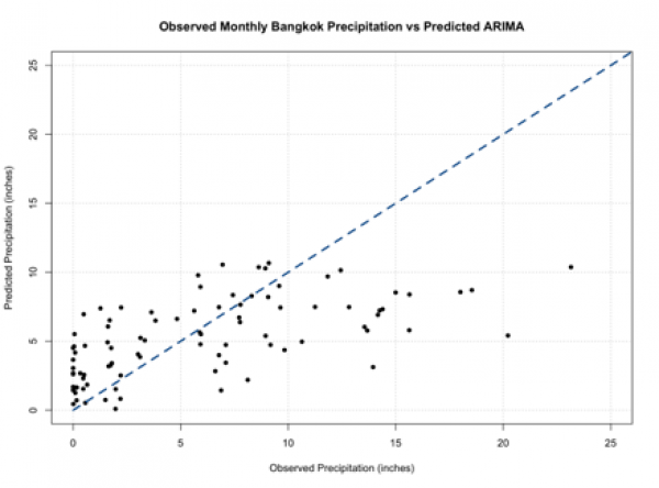
You should note that these predictions do not stem from the same model and can have different parameters (p,q) for each prediction. If you compare this to our other plots from a pure AR and pure MA model, you will see it’s not much different. So, we haven’t really improved the skill of the model.
Periodic ARIMA Example
One of the reasons why we haven’t improved the model may be due to the quasi-periodicity that exists in the dataset. Look back at the ACF for the data:
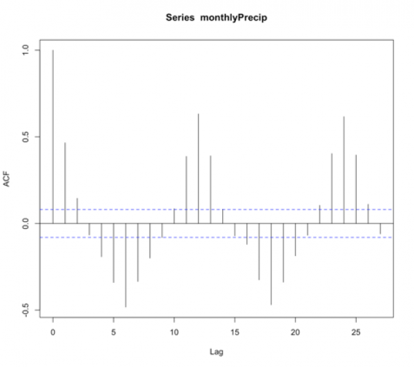
We see high values at fixed intervals. Consulting our summary table from before:
| Shape | Model |
|---|---|
| Exponential, Decaying to Zero | AR model: use PACF to identify the order |
| Alternating positive and negative, decaying to zero | AR model, use PACF to identify the order |
| One or more spikes, rest are at 0 | MA model, order identified by the lag at which the correlation becomes zero |
| Decay starting after a few lags | ARMA |
| All 0 or close to 0 | Data is random |
| High values at fixed intervals | Include seasonal AR term |
| No Decay to 0 | Series is not stationary (possible trend or periodicity)- include differencing term |
We need to include a seasonal term. Unfortunately, we can’t just supply the data to the ‘auto.arima’ function and let it do its magic. Instead, we need to create a time series function that creates this seasonal term. So let’s give this a try. To start, we need to look at the ACF to make a first guess at the periodicity. We see the strong positive correlation at lag 1, then again at lag 12 and lag 24. This is suggesting a strong annual periodicity. We will start by setting M to 12 (12 months in a year; we are working with monthly data), and we will create a time series object with the frequency set to 12.
Your script should look something like this:
# create a time series object
precipTS <- ts(monthlyPrecip, frequency=12)
The ‘ts’ function creates a time series object with a specified frequency for each time. So in this case, I said the frequency is 12, and it pulls out the observations every 12 months - which corresponds to the periodicity we saw in the ACF. Now we run the ‘auto.arima’ function and tell it to include a seasonal component.
Your script should look something like this:
# create Periodic ARIMA model
precip_PeriodicARIMA <- auto.arima(precipTS,ic="aic",seasonal=TRUE)
The printout tells us an ARIMA(2,0,0)(2,0,0)[12] was selected. So let’s review what this means. It’s an ARIMA model with p order of 2, d order of 0, and q order of 0 - meaning it’s an AR model of order 2. With a periodic ARIMA model of P order 2, D order 0, and Q order 0, meaning it’s a periodic AR model of order 2, and the periodicity is 12 months ([12]). If we run the summary function, we see that the RMSE is 3.55 inches. Now, if we wanted to automate the decision of the periodicity ([m]), we can use the following algorithm.
Your script should look something like this:
# automate the frequency
AICScore <- {} for(i in 1: 24){
  # create a time series object
  precipTS <- ts(monthlyPrecip,frequency=i)

  # create Periodic Arima Model
  precip_PeriodicARIMA <- auto.arima(precipTS,ic="aic",seasonal=TRUE)

  # save the AIC score
  AICScore[i] <- precip_PeriodicARIMA$aic
}
This is a very simple algorithm that saves the AIC score for the best ARIMA model with each periodicity [1:24]. Now we can look at the 'AICScore' and find the best model by minimizing the AIC.
Your script should look something like this:
# select optimal frequency choice
optimalFrequency <- which(min(AICScore) == AICScore)
We see that the optimal frequency is 12, which is what we previously selected, and confirms our observations in the ACF. So, now let’s automate the model to update after each observation. We can then predict the values and compare the observations to predictions.
Your script should look something like this:
# predict values
precipARIMA_predict<-{}
for(i in 1:100){
  # subset data
  dataSubset <- monthlyPrecip[(i:(length(monthlyPrecip)-101+i))]

  # create a time series object
  precipTS <- ts(dataSubset,frequency=12)
  precip_ARIMA <- auto.arima(precipTS,ic="aic",seasonal=TRUE, allowdrift=FALSE)
  precipARIMA_predict[i] <- predict(precip_ARIMA,n.ahead=1)$pred
}
As a reminder, each prediction was created with a unique model that potentially has different p,d,q and P, D, Q parameters. The added parameter here, 'allowdrift', tells the function to not include any drift (e.g., long term changes in data) in the model. Let’s plot the results.
Your script should look something like this:
# plot predicted and observed values
dataObserved <- monthlyPrecip[(length(monthlyPrecip)-99):length(monthlyPrecip)]
precipARIMA_predict[which(precipARIMA_predict <0)] <- NA
plot.new()
grid(nx=NULL,ny=NULL,'grey')
par(new=TRUE)
plot(dataObserved,precipARIMA_predict,xlab="Observed Precipitation (inches)",
     ylab="Predicted Precipitation (inches)",main="Observed Monthly Bangkok Precipitation vs Predicted Periodic ARIMA",
     xlim=c(0,25),ylim=c(0,25),pch=16)
par(new=TRUE)
plot(seq(0,30,1),seq(0,30,1),type='l',lty=2,col='dodgerblue4',lwd=3,xlab="Observed Precipitation (inches)",
     ylab="Predicted Precipitation (inches)",main="Observed Monthly Bangkok Precipitation vs Predicted Periodic ARIMA",
     xlim=c(0,25),ylim=c(0,25))
You should get a figure like this:
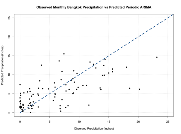
Out of all our figures, this one seems to be the best fit, following the 1-1 line better than the previous models.
ARIMA and Periodic ARIMAs are great because they are computationally efficient, easy to update, and are based on historical patterns. But they tend to not capture extreme values, and cannot model complex relationships. Nonetheless, these models are important steppingstones to more robust and complex models that we will learn about later on.