The Gibbs Phase Rule relates the degrees of freedom in a system to the number of components and number of phases in a system. The Gibbs Phase Rule is:
Where:
F the number of degrees of freedom in the system, integer
C is the number of components in the system, integer
P is the number of phases in the system, integer
The use of the Gibbs Phase Rule is best illustrated with examples; however, to do this we must first discuss some fundamental thermodynamic concepts. The phrase “degrees of freedom” refers to the maximum number of independent thermodynamic variables (pressure, temperature, and intensive variables) that you can vary simultaneously within a system at equilibrium before you are forced to specify one or more of the remaining variables (or disturb the equilibrium of the system). By “intensive variables”, we are referring to variables that are independent of the size of the system. For example, phase density in a system is an intensive variable because you can halve the size of the system, and the phase density will remain the same. On the other hand, the mass of a system is an extensive property because if you halve the size of the system, then you halve the mass in the system. A component refers an individual chemical element that exists in the system (in our case, a molecular species: methane, ethane, cyclopentane, benzene, CO2, H2O, etc.). Finally, a phase is a physical state of matter with homogenous (uniform) composition, physical properties, and chemical properties. In petroleum and natural gas engineering, we typically deal with systems containing four phases: a gaseous hydrocarbon phase (natural gas), a liquid hydrocarbon phase (crude oil), a liquid aqueous phase (water or brine), and a solid rock phase. There are times when we deal with systems containing more phases (such a solid hydrocarbon phase or multiple hydrocarbon liquid phases), but the circumstances when this occurs are beyond the scope of this class.
For a single-component system, we have C = 1, and Gibbs Phase Rule becomes:
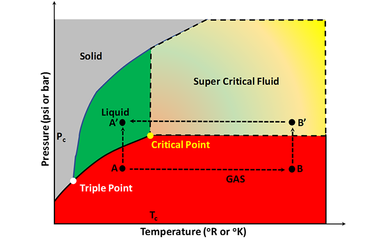
If we were to plot the phase state (number and types of phases) on a pressure-temperature plot for this single-component system, then we would obtain a plot like that shown in Figure 2.09. This figure is also referred to as a Phase Diagram or a P-T Diagram. In this Phase Diagram, the grey region represents all of the pressure-temperature combinations that result in the solid form of our single component, the green region represents the pressure and temperature combinations that result in the liquid form of our single component, the red region represents the pressure and temperature combinations that result in the gaseous form of our single component, and the multi-colored region represents the super critical form of our single component. Also posted on this Phase Diagram are two points, the triple point and the critical point.
Getting back to the single component version of the Gibbs Phase Rule, Equation 2.04, we can start to clarify some of the concepts that we have already discussed with some examples. If we consider the single-phase regions in Figure 2.09 (P = 1 in Equation 2.04), then from Equation 2.04, we have 2 degrees of freedom (F = 2). This implies that we can independently vary Pressure and Temperature within the Phase Envelope (colored regions) and not change the phase state of the system. In other words, two degrees of freedom represent two-dimensional regions (areas) on the Phase Diagram in which a single phase exists.
Now, let’s consider the occurrence of two phases coexisting simultaneously (P = 2) in equilibrium. From Equation 2.04 with P = 2, we have one degree of freedom (F = 1). In Figure 2.09, we have two coexisting phases along the borders of the phase envelopes. For example, the line bordering the Solid and Liquid Phases represents the pressure-temperature conditions where the solid form of our single component system can coexist with the liquid form of our single component at equilibrium (think of polar caps sitting on water near the earth’s poles). For two phases to coexist in equilibrium, if we were to change one variable, say temperature, then we would be forced to change pressure in a manner that it remained on the border line between the two single-phase regions. In other words, one degree of freedom represents the one-dimensional, curvilinear lines which act as borders between the single-phase regions. If we change one variable on one of these border lines, then we are forced to change the other variable to remain on the border line.

Finally, we can consider the coexistence of three phases (P = 3 in Equation 2-4) in a system at equilibrium. From Equation 2.04 with P = 3, we have F = 0, or no degrees of freedom. This implies that at the point where three phases coexist (the Triple Point in Figure 2.09), we cannot change either pressure or temperature and retain a three-phase system in equilibrium of the single-component (pure) system. The Triple Point is a property of the component that we are considering. Thus, zero degrees of freedom refers to a 0-Dimensional point (the Triple Point)
In Figure 2.09, the Critical Point is also plotted. The Critical Point, defined by the critical pressure, Pc, and the critical temperature, Tc: (Pc, Tc) is the point in the system that defines the onset of the super critical state. Super critical fluids are fluids in which the gaseous phase becomes indistinguishable from the liquid phase (the phase densities become equal).
Consider a pressure-temperature pair in the single-phase gas region with a temperature somewhere between the temperature at the triple point and the critical temperature, Tc, such as Point A in Figure 2.10. If we were to increase the pressure of this single-phase gas (Path A-A’), then we would see a distinct and abrupt change in the phase state of the fluid as we crossed into the single-phase liquid region. This is because the densities of the gaseous phase and the liquid phase are different. Now, if we were to do the same experiment starting at a temperature greater the critical temperature, Tc, such as Point B, then as we increased the pressure on the single-phase gas (Path B-B’) and entered the Super Critical Fluid region, there would be no abrupt phase change.
We could also perform a third experiment where we started at the original point, Point A, and followed the pressure-temperature path Path A-B-B’-A’ into the single-phase liquid region to arrive at Point A’. In this last experiment, we would arrive at the same point, Point A’, as in the first experiment, but without any abrupt phase change. The system properties would change smoothly and continuously during the entire experiment.
For multi-component systems like real crude oil – natural gas systems, the Pressure-Temperature Diagram is much more complex. This is because a real crude oil – natural gas system may contain tens or hundreds of thousands of components. For Multi-Component Systems, the P-T Diagram looks like that in Figure 2.11. A Phase Diagram, such as that shown in this figure, typically is measured in the laboratory but can also be generated mathematically with sophisticated models, such as, Cubic Equation of State Equations (multi-component extensions to van der Waal’s Equation).
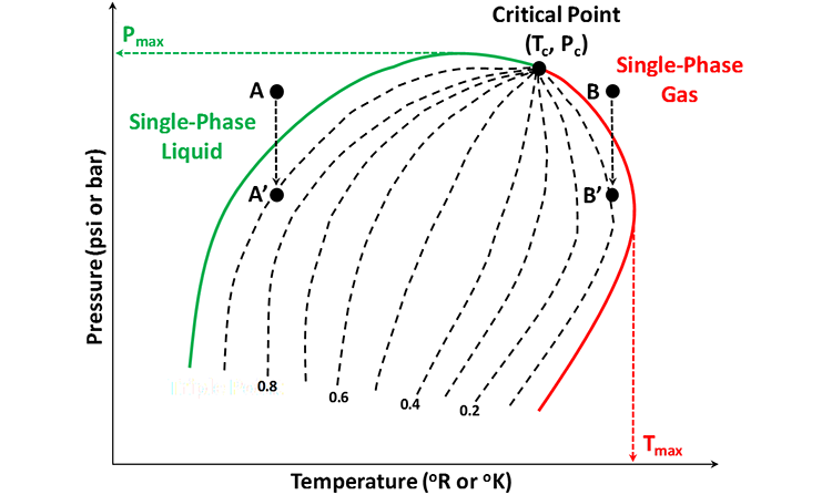
In this figure, the region between the green curve and the red curve is the two-phase envelope; while the region outside of the two-phase envelope is the single-phase region. Single-phase liquids exist to the left (lower temperatures) and above (higher pressures) the bubble-point locus (green curve); while single-phase gases exist to the right (higher temperatures) of the dew-point locus (red curve).
The green curve in this figure represents the Bubble-Point Locus of this multi-component system; the red curve represents the Dew Point Locus of the system, and the dashed lines in the two-phase region represents the quality lines of the system (lines of constant volume-fraction of the liquid phase). The bubble-point, defined by a bubble-point pressure, Pb and a bubble-point temperature, Tb, is the point on a pressure-temperature path (originating in the single-phase liquid region) where the path enters the two-phase region (crosses the green curve in Figure 2.11). The name “bubble-point” comes from the fact that this is the point where the first bubble of gas evolved from a liquid as it enters the two-phase region. For example, Point A in Figure 2.11 lies in the single-phase liquid region. As the pressure is reduced at a constant temperature (isothermal conditions), it follows the Path A-A’. The point where Path A-A’ enters the two-phase region (crosses the green, bubble-point locus) represents the bubble-point pressure for this temperature. This is the point where the first bubble of gas is formed in the system. The pressure reduction is continued until it terminates at Point A’. Point A’ lies on the 0.9 quality line, implying that at this point, the system is composed of two-phases with the liquid phase occupying 90 percent of the volume.
On the other hand, the dew-point, defined by the dew-point pressure and dew-point temperature is the point on a pressure-temperature path (originating in the single-phase gas region) enters the two-phase region. The name dew-point refers to the point where the first liquid drop condenses from the gaseous phase. For example, Point B in Figure 2.11 lies in the single-phase gas region and enters the two-phase region when the pressure is reduced under isothermal conditions (Path B-B’). The dew point pressure for this temperature then is the pressure where Path B-B’ crosses the red dew-point locus. If the isothermal pressure reduction is stopped at Point B', then the system at equilibrium will contain two phases with the liquid phase occupying 10 percent of the system volume.
Finally, the pressure, Pmax in Figure 2.11 is the cricondenbar (the maximum pressure in which two phases can coexist); while the temperature, Tmax is the cricondentherm (the maximum temperature in which two phases can coexist).
With these preliminary concepts, we can now continue with our discussion on the types of hydrocarbon reservoirs encountered in the oil and gas industry.