Among contrarians in the public debate about climate change, one often hears an argument that goes something like this:
"Sure, the climate is changing. But climate is always changing. It was warmer than today in the past due to natural causes! So the warmth today could also be due to natural causes?"
Is this a legitimate argument? Well, we began to address the issue back during our introduction to the concept of climate change. Let's explore the issue in more detail now, looking at what observations are available to document (a) how climate changed in the past and (b) what factors appear to have been responsible for those changes.
Geological Variations
Let's start out with a look at the longest timescale changes that are documented in the geological record. We're talking hundreds of millions of year timescales. While the records are imperfect at best, we do have a rough idea from very old sedimentary records as to the broad-scale changes in global temperatures and in atmospheric CO2 over these timescales. On these very long timescales, the changes in atmospheric CO2 are related to geologic processes such as plate tectonics, which govern the outgassing of CO2 from Earth's interior by volcanoes, and the slow changes in Earth's continental configuration and relief, which influence natural processes such as chemical and physical weathering that take CO2 out of the atmosphere.
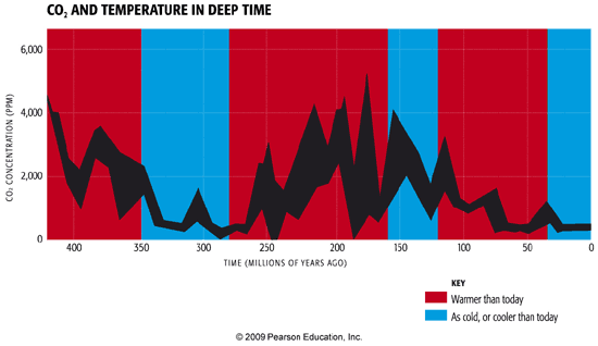
Its quite clear from the comparison above that, on these long timescales, atmospheric CO2 levels and global temperatures appear to be very closely correlated. Warm periods, with some exceptions, are periods of high atmospheric CO2, and cold periods, geologically, have been periods of low atmospheric CO2. You can hear Penn State professor Richard Alley's eloquent Bjerknes Lecture on the subject at the 2009 meeting of the American Geophysical Union.
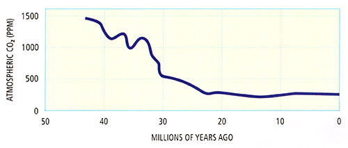
Let's zoom in further over the past 50 million years.
© 2015 Pearson Education, Inc.
This interval takes us from the warm early Eocene period, to the cooler Miocene period, and eventually to the Plio-Pleistocene period of the past 5 million years, during which large-scale glaciation of the modern continents was first observed. We see that this transition from a warm to glacial climate was accompanied by a major decrease in atmospheric CO2 levels.
The decrease in atmospheric CO2, once again, doesn't explain all of the details of course. For example, CO2 appears relatively flat for the final two million years, even as the climate continues to have cooled through the Plio-Pleistocene transition. Some of that cooling may represent positive ice albedo feedbacks that kick in once large-scale glacial inception takes hold over the past 20-30 million years. Nonetheless, CO2 clearly remains the major knob controlling global climate over the past 50 million years. Once we zoom in on yet shorter timescales, that is tens of thousands of years, we see that another dynamic appears to have been at play.
Glacial/Interglacial Variations
Once we enter into the Pleistocene period of the past 1.5 million years, large-scale glaciation of the Northern Hemisphere takes hold, but there are prominent alternations between relatively ice-covered periods (the "Ice Ages"), and warmer periods more similar to modern, pre-industrial conditions. It is instructive to consider what factors appear to have been driving these variations.
Pleistocene Ice Ages
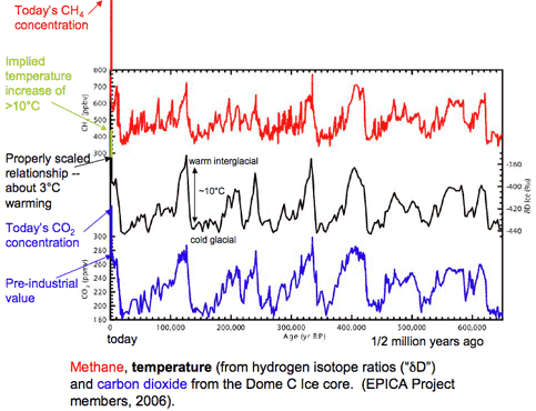
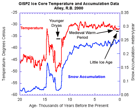
For nearly the past million years, CO2 concentrations, as recorded in Antarctic ice cores, have oscillated by roughly 100 ppm, alternating between low glacial levels of roughly 180 ppm and relatively high interglacial levels of roughly 280 ppm. Methane (CH4) concentrations oscillate by nearly a factor of two as well. And temperatures in Antarctica, as recorded by oxygen isotopes in the ice cores, have varied in concert with these greenhouse gas concentrations changes. If one takes into account the typical polar amplification of warming, the peak-to-peak changes in temperature in Antarctica (roughly 10°C) translate to a change in global mean temperature of about 3°C. At least half of that temperature change is due to changes in Earth's albedo (reflectivity) associated with the changes in surface ice cover. That leaves the remaining 1.5°C temperature change to be explained by the changes in greenhouse gas concentrations (CO2 and also CH4). If we work out the implied sensitivity of the global climate to greenhouse gas concentrations, it implies a value that lies within the typical range of estimates, i.e., between 1.5° and 4.5°C for a doubling of CO2 concentrations. (You can read more about the details of this argument in The lag between temperature and CO2 article from Real Climate).
But why do the oscillations occur? Why do they have a roughly 100,000 year ('100 kyr') periodicity? And why is the shape of the oscillation not a sinusoidal cycle, but a "sawtooth" waveform with a slow, long-term descent into glacial conditions and a very rapid termination? These features certainly require further explanation.
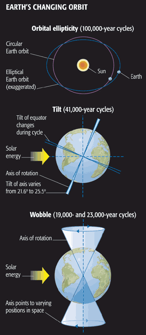
The pacing of the 100 kyr oscillation is almost certainly tied to long-term changes in Earth orbital geometry. As I alluded to in the introductory lecture of the course, the geometry of Earth's annual orbit around the Sun changes slowly over time. These changes are subtle, but they are persistent over thousands of years and have a profound impact on climate.
The first of these orbital variations involves the very slow wobble (or to use the more technical term, the precession) of the Earth's rotational axis. One full wobble (analogous to the wobbling of a gyroscope—see animation below) takes roughly 19-23 kyr. The precession determines when the Northern and Southern Hemisphere are each tilted toward (summer) or away (winter) from the Sun.

The primary importance of this factor is that it determines whether the summer solstice in a given hemisphere occurs when Earth is farthest (making summer a little cooler) or closest (making summer a little warmer) to the Sun. This factor only matters, then, because Earth's annual orbit around the Sun is not circular, but slightly elliptical - a factor discussed further below.
The second of these changes involves the tilt angle (or to use the more technical term, the obliquity) of Earth's orbit. The Earth's rotational axis today is inclined at an angle of roughly 23.5 degrees from the vertical (this is the angle of the precessing top shown in the animation above). This is why the tropics are located at 23.5N and 23.5S and why the Arctic and Antarctic circles are located at 90-23.5 = 66.5 N and S respectively. This angle of inclination is not fixed over time, however. It varies between roughly 21.5 degrees and 25.5 degrees. Seasonality only exists because of the tilt; if not for the tilt, neither hemisphere would be preferentially tilted towards the Sun at any time of the year. Therefore, periods when the tilt angle is greatest are periods of heightened seasonality, while periods when the tilt angle is smallest have reduced seasonality. It takes roughly 41 kyr for the tilt angle to go through one full cycle of alternation between lesser and greater values of the obliquity.
The final of the changes involves the ellipticity (or, to use the more technical term, the eccentricity) of the orbit. Earth's orbit around the Sun is not circular, but, instead, is slightly elliptical. The degree of ellipticity is measured by the eccentricity, which ranges from roughly zero (an essentially circular orbit) to a maximum of roughly 4% (a very slightly elliptical orbit). It takes roughly 100 kyr for the eccentricity to go through one full cycle of alternation between low and high eccentricity.
This might sound like the smoking gun to explain the dominant 100 kyr periodicity of the ice ages. But it's not quite that simple.
The changes in insolation associated with the 100 kyr eccentricity variations is considerably smaller than the shorter (19-23 kyr and 41 kyr) precession and obliquity periodicities. And prior to about 700,000 years ago, the glacial/interglacial cycles were dominated by these shorter periodicities. So what is it that is responsible for the dominant 100 kyr oscillation of the past 700,000 years?
To understand this, we have to think a bit more about how these various effects interact. The precession and obliquity don't actually change the net solar radiation at the top of the atmosphere; they simply redistribute it with respect to season and latitude. The eccentricity, however, does change the net solar radiation. When Earth's orbit is more elliptical, it spends more time over the course of a year being relatively far away from the sun, and thus there is a decrease in the received solar radiation. Because the change is very small, however, it's necessary to have large amplifying feedbacks to give this effect a greater role.
Think About It!
Any guess as to what feedbacks may do the trick?
Click for answer.
The ice-albedo feedback is key to understanding the glacial/interglacial cycles. While this feedback is a moderate player in the context of modern climate change (responsible, for example, for only about 0.6°C of the 2.5-3°C warming expected for a doubling of CO2 concentrations), it is considerably more important during ice ages, when continental ice sheets reached as far south as New York City.
This observation provides a clue as to how the 100 kyr periodicity emerges when the actual radiative forcing at the 100 kyr timescale is so weak. Roughly every 100 kyr or so, the eccentricity reaches a particularly high value, favoring the largest possible differences in Earth-Sun distance over the course of the annual cycle. During such times, there will be a point over the course of the much faster 19-23 kyr precession cycle, where the Northern Hemisphere winter solstice will coincide with the minimum Earth-Sun distance ('perihelion'), and the summer solstice will coincide with the maximum Earth-Sun distance ('aphelion'). This makes winters at high northern latitudes unusually warm and summers at high northern latitudes unusually cool. Such conditions are ideal for growing ice sheets: the warm winters actually allow for greater amounts of snowfall (since warm winter air holds more moisture than cold winter air), and the cool summers help prevent any accumulated winter snow from melting over the course of the summer. Ice begins to accumulate, more solar radiation is reflected to space, and the cooling spreads southward. Pretty soon, you've got a full-fledged ice age on your hands. This effect, of course, is enhanced when the obliquity is greatest.
So, we can see how all three factors—the eccentricity, the precession, and the obliquity—work together to create ice ages. But the thing that appears to trigger it all is the slow, 100 kyr eccentricity forcing, since high eccentricity—reached roughly every 100 kyr—sets up the perfect storm of conditions for establishing an ice age. Once those conditions occur, an ice age slowly sets in and builds, for tens of thousands of years. This is the slow descent into the ice ages seen in the ice core figure earlier. Eventually, however, as we near 100 kyr from the starting point, the eccentricity again rises to high levels. Then, when the faster precession cycle reaches a point where seasonality is enhanced rather than diminished, ie., northern summers are especially warm—the ice begins to melt, and the positive ice-albedo feedback kicks in in an especially dramatic fashion, yielding the rapid warming that defines the abrupt termination evident in the ice core figure.
The mechanism described below requires the possibility of building large ice sheets. It is widely speculated that the climate had to cool beyond some threshold where large ice sheets could grow, and that the slow cooling was provided by the gradual lowering of CO2 concentrations over the course of the Pleistocene. Eventually, the climate cooled to that point, and the 100 kyr oscillations ensued.
And what about the role of CO2 in all of this? As I noted above, CO2 is clearly an important player. We cannot explain the extent of the warming and cooling over the glacial/interglacial cycles without including the direct warming effect of CO2. But the situation is somewhat more complicated than that since CO2 is not simply a control variable on these timescales. The global carbon cycle (in particular the oceanic carbon cycle) is changing in response to the climate changes taking place. For example, a warming ocean favors outgassing of CO2 into the atmosphere, which of course amplifies the warming further because of the greenhouse effect.
So CO2 is acting both as a forcing and as feedback. That is different from the current situation, where we essentially have our hands on the CO2 knob of the system (though, even here, there are some complications, as we will discuss in more detail in Lesson 6 on carbon emission scenarios).
The Younger Dryas
At the termination of the last ice age, roughly 12 kyr ago, something surprising happened. Just as Earth appeared to be coming out of the ice age, it staged a reversal and headed back into glacial conditions for at least 1000 years. The cooling event seems to have been centered in the North Atlantic ocean. This episode is known as the Younger Dryas (named after the spread of the tundra-loving Dryas flower, whose range during this time interval plunged southward in regions surrounding the North Atlantic ocean).
While there is still some scientific debate about the details, it is generally believed that this rapid cooling resulted from a slowdown or collapse of the ocean's thermohaline circulation in response to the massive flux of freshwater into the high-latitude North Atlantic as the Northern Hemisphere ice sheets and glaciers rapidly began to melt. This fresh water would have inhibited the sinking motion that typically occurs in the sub-polar regions of the North Atlantic, suppressing the overturning circulation associated with the North Atlantic drift current which helps to warm the high-latitudes of the North Atlantic and surrounding regions.
It is, in fact, this event from the distant past that has given rise to the popular, if rather flawed (as we will see when we look at actual climate projections), concept that global warming may ironically lead to another ice age. This concept was caricatured in the movie 'The Day After Tomorrow'. The problem with the analogy is that there isn't nearly the amount of ice around today to melt that there was at the termination of the last ice age, and thus the effect is likely to be much smaller. As we will see later in the course, however, there may be a very small grain of truth to the scenario laid out in the movie.
The Holocene
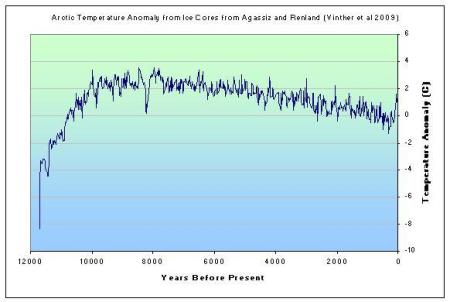
Even during interglacial intervals, when there is relatively little ice around, the higher-frequency orbital forcings still have an influence on climate. In particular, the impacts of the roughly 19-23 thousand year precession cycle are evident over the course of the current interglacial period of the past 12,000 years known as the Holocene. Today, precession has the effect of minimizing Northern Hemisphere seasonality, since perihelion occurs very close (January 3) to the winter solstice (Dec 22nd). Roughly 1/2 of a precession cycle (i.e., about 11,000 years) ago, precession had the effect of maximizing Northern Hemisphere seasonality. Indeed, it was this exaggerated seasonality that helped end the last ice age by favoring summer melting. Over the next 12,000 years, the seasonal pattern of insolation slowly evolved to what it is today.
If we look at temperature estimates based on oxygen isotopes from Arctic ice cores, we find that summer temperatures were relatively high during a period sometimes called the Holocene optimum that lasted from about 10,000-6,000 years ago, before slowly declining towards pre-industrial levels (and then spiking again over the last 100 years—something we'll discuss more below). This pattern of high-latitude summer temperature change is precisely what we expect, given the precession changes discussed above. On the other hand, tropical insolation was actually reduced, as was winter insolation at higher northern latitudes. That makes these natural past changes in radiative forcing very different from those associated with modern greenhouse increases which are positive during both seasons, in both hemispheres, and in the tropics as well as high latitudes.
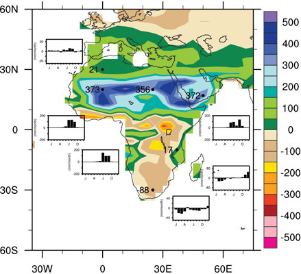
As the seasonal and latitudinal pattern of solar heating evolved over the course of the Holocene, so did the atmospheric circulation which is driven in substantial part by those variations in heating. For example, paleoclimate evidence suggests that the Sahara desert was considerably more lush than today, supporting steppe vegetation and large lakes that were home to crocodiles and hippopotamuses. Simulations with climate models, forced by the known changes in seasonal insolation, reproduce this pattern, as a consequence of strengthened west African monsoon, driven by the larger seasonal changes in insolation.
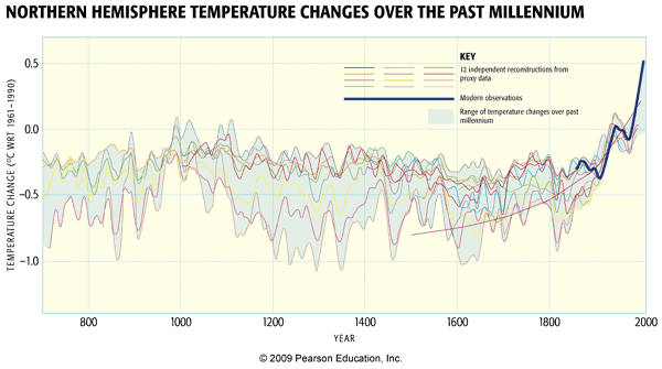
The Past 1,000 Years
Over the past 1,000 years, changes in insolation due to Earth orbital effects are relatively small. The primary natural radiative forcings believed to be important on this time frame (as we will see in Lesson 5 when we talk about Estimating Climate Sensitivity) are volcanic eruptions and changes in solar output.
The basic 'boundary conditions' on the climate (distribution of ice sheets, orbital geometry, continental configuration, etc.) were essentially the same as they are today, making this a useful interval to study from the standpoint of modern climate change. The pre-industrial interval of the past 1,000 years forms a sort of 'control', as the only real difference from today is the added impact over the past century or two of human influence on climate. Some (in particular, the atmospheric chemist Paul Crutzen, who won the Nobel Prize for his work on the stratosphere ozone hole) have argued that the period since the dawn of industrialization (i.e., the past two centuries) has been impacted substantially enough already by human activity that we should consider it as a distinct interval separate from the current interglacial, i.e., that we are no longer in the Holocene, but rather, an entirely new, human-created interval of Earth history known as the anthropocene.
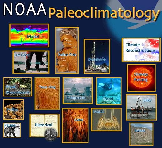
Patterns of surface temperature can be estimated in past centuries from "proxy" records such as tree-rings, corals, ice cores, faunal remains and other sources. For more information about the work that Michael Mann has done on this topic, you might check out an Interactive Presentation of the Global Temperature Patterns in Past Centuries.
Looking at the temperature patterns reconstructed from these proxy records, we can gain a longer-term perspective on the natural climate variability associated with ENSO, and the NAO, and other known dynamical patterns influencing the climate system. Can you spot some big El Niño events in the 18th century? What about the effect of the NAO—can you discern that in the patterns? How?
If we average over these patterns (focusing on the Northern Hemisphere, since information in the Southern Hemisphere is limited) , we can obtain an estimate of the average temperature in past centuries. There are numerous reconstructions that have been performed of this sort, using different types of proxy data, and different statistical approaches to estimating temperatures from the data. But one thing they all have in common is finding that the recent warming is anomalous as far back as these reconstructions go (more than 1,000 years now).
Does this mean that the warming is due to human activity? No—it's possible that the warming could just be a fluke of nature. To assess whether or not the recent warming can be attributed to human activity, we'll need to turn to theoretical climate models - the topic of our next lesson!