1.3.2 Opening and exploring ModelBuilder

Let’s get some practice with ModelBuilder to solve a real scenario. Suppose you are working on a site selection problem where you need to select all areas that fall within 10 miles of a major highway and 10 miles of a major city. The selected area cannot lie in the ocean or outside the United States. Solving the problem requires that you make buffers around both the roads and the cities, intersect the buffers, then clip to the US outline. Instead of manually opening the Buffer tool twice, followed by the Intersect tool, then the Clip tool, you can set this up in ModelBuilder to run as one process.

1. Create a new Pro project called Lesson1Practice in the C:\PSU\Geog485\Lesson1 folder.
2. Add the us_cities, us_roads, and us_boundaries shapefiles from the Lesson 1 data folder that you configured previously in this lesson to a new map.
3. In the Catalog pane, right-click your Lesson1Practice toolbox and click New > Model.  You’ll see ModelBuilder appear in the middle of the Pro window.
4. Under the ModelBuilder tab, click the Properties button.
5. For the Name, type SuitableLand and for the Label, type Find Suitable Land. The label is what everyone will see when they open your tool from the Catalog. That’s why it can contain spaces. The name is what people will use if they ever run your model from Python. That’s why it cannot contain spaces.

6. Click OK to dismiss the model Properties dialog.

   You now have a blank canvas on which you can drag and drop the tools. When creating a model (and when writing Python scripts), it’s best to break your problem into manageable pieces. The simple site selection problem here can be thought of as four steps:

   • Buffer the cities
   • Buffer the roads
   • Intersect the buffers
   • Clip to the US boundary

   Let’s tackle these items one at a time, starting with buffering the cities.

7. With ModelBuilder still open, go to the Catalog pane > Geoprocessing tab and browse to Analysis Tools > Proximity.

8. Click the Buffer tool and drag it onto the ModelBuilder canvas. You’ll see a gray rectangular box representing the buffer tool and a gray oval representing the output buffers. These are connected with a line, showing that the Buffer tool will always produce an output data set.

   In ModelBuilder, tools are represented with boxes and variables are represented with ovals. Right now, the Buffer tool, at center, is gray because you have not yet supplied the required parameters. Once you do this, the tool and the variable will fill in with color.

9. In your ModelBuilder window, double-click the Buffer box. The tool dialog here is the same as if you had opened the Buffer directly from the Catalog pane. This is where you can supply parameters for the tool.
10. For Input Features, browse to the path of your us_cities shapefile on disk. The Output Feature Class will populate automatically.
11. For Distance [value or field], enter 10 miles.
12. For Dissolve Type, select Dissolve all output features..., then click OK to close the Buffer dialog. The model elements (tools and variables) should be filled in with color, and you should see a new element to the left of the tool representing the input cities feature class.

13. An important part of working with ModelBuilder is supplying clear labels for all the elements. This way, if you share your model, others can easily understand what will happen when it runs. Supplying clear labels also helps you remember what the model does, especially if you haven’t worked with the model for a while.

    In ModelBuilder, right-click the us_cities.shp element (blue oval, at far left) and click Rename. Name this element "US Cities."

14. Right-click the Buffer tool (yellow-orange box, at center) and click Rename. Name this “Buffer the cities.”

15. Right-click the buffer output element (green oval, at far right) and click Rename. Name this “Buffered cities.” Your model should look like this.  

    

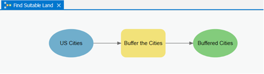    Figure 1.2 The model's appearance following step 15, above.
16. Save your model (ModelBuilder tab > Save). This is the kind of activity where you want to save often.

17. Practice what you just learned by adding another Buffer tool to your model. This time, configure the tool so that it buffers the us_roads shapefile by 10 miles. Remember to set the Dissolve type to Dissolve all output features... and to add meaningful labels. Your model should now look like this.  

    

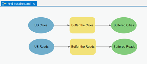    Figure 1.3 The model's appearance following step 17, above.
18. The next task is to intersect the buffers. In the Catalog pane's list of toolboxes, browse to Analysis Tools > Overlay and drag the Intersect tool onto your model. Position it to the right of your existing Buffer tools.
19. Here’s the pivotal moment when you chain the tools together, setting the outputs of your Buffer tools as the inputs of the Intersect tool. Click the Buffered cities element and drag over to the Intersect element. If you see a small menu appear, click Input Features to denote that the buffered cities will act as inputs to the Intersect tool. An arrow will now point from the Buffered cities element to the Intersect element.
20. Use the same process to connect the Buffered roads to the Intersect element. Again, if prompted, click Input Features.

21. Rename the output of the Intersect operation "Intersected buffers." If the text runs onto multiple lines, you can click and drag the edges of the element to resize it. You can also rearrange the elements on the page however you like. Because models can get large, ModelBuilder contains several navigation buttons for zooming in and zooming to the full extent of the model in the View button group on the ribbon.  Your model should now look like this:

    

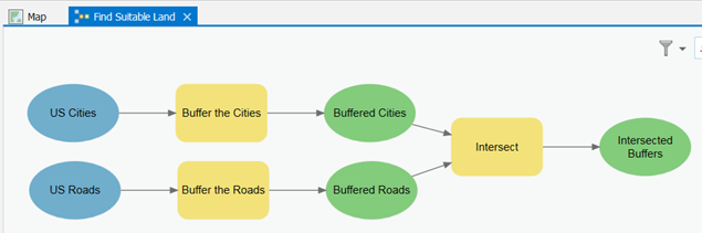    Figure 1.4 The model's appearance following step 21, above.
22. The final step is to clip the intersected buffers to the outline of the United States. This prevents any of the selected area from falling outside the country or in the ocean. In the Catalog pane, browse to Analysis Tools > Extract and drag the Clip tool into ModelBuilder. Position this tool to the right of your existing tools.
23. As you did above, set the Intersected buffers as an input to the Clip tool, choosing Input Features when prompted. Notice that even when you do this, the Clip tool is not ready to run (it’s still shown as a gray rectangle, located at right). You need to supply the clip features, which is the shape to which the buffers will be clipped.
24. In ModelBuilder (not in the Catalog pane), double-click the Clip tool. Set the Clip Features by browsing to the path of us_boundaries.shp, then click OK to dismiss the dialog. You’ll notice that a blue oval appeared, representing the Clip Features (US Boundaries).

25. Set meaningful labels for the remaining tools as shown below. Below is an example of how you can label and arrange the model elements.

    

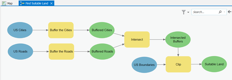    Figure 1.5 The completed model with the clip tool included.
26. Double-click the final output element (named "Suitable land" in the image above) and set the path to C:\PSU\Geog485\Lesson1\suitable_land.shp. This is where you can expect your model output feature class to be written to disk.
27. Right-click Suitable land and click Add to display.
28. Save your model again.
29. Test the model by clicking the Run button. You’ll see the by-now-familiar geoprocessing message window that will report any errors that may occur. ModelBuilder also gives you a visual cue of which tool is running by turning the tool red. (If the model crashes, try closing ModelBuilder and running the model by double-clicking it from the Catalog pane. You'll get a message that the model has no parameters. This is okay [and true, as you'll learn below]. Go ahead and run the model anyway.)

30. When the model has finished running (it may take a while), examine the output on the map. Zoom into Washington state to verify that the has Clip worked on the coastal areas. The output should look similar to this.

    

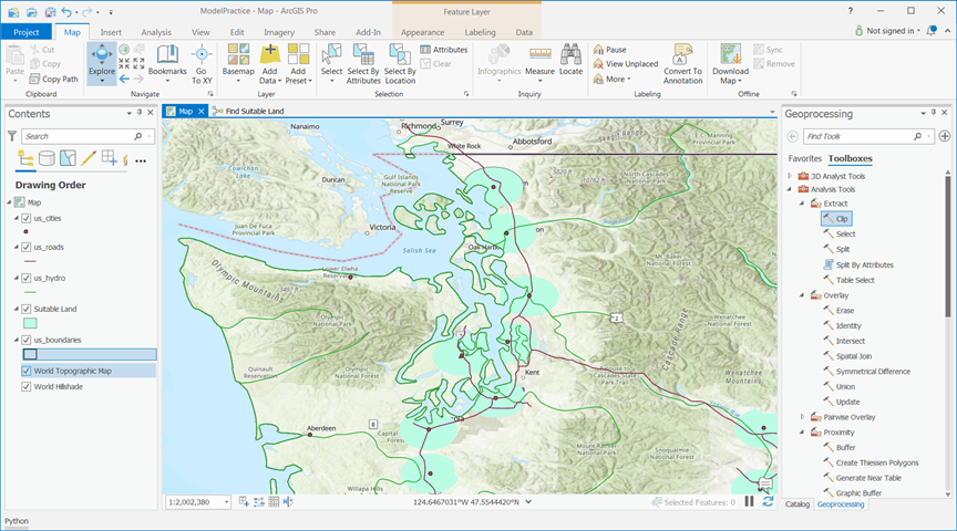    Figure 1.6 The model's output in ArcGIS Pro.

That’s it! You’ve just used ModelBuilder to chain together several tools and solve a GIS problem.

You can double-click this model anytime in the Catalog pane and run it just as you would a tool. If you do this, you’ll notice that the model has no parameters; you can’t change the buffer distance or input features. The truth is, our model is useful for solving this particular site-selection problem with these particular datasets, but it’s not very flexible. In the next section of the lesson, we’ll make this model more versatile by configuring some of the variables as input and output parameters.