Project 5: Examine Relationships in Data: Regression Diagnostic Utilities: Checking Assumptions

As was discussed earlier, regression analysis requires that your data meet specific assumptions. Otherwise, the regression output may not be meaningful. You should test those assumptions through statistical means. These assumptions can be assessed through RStudio.

Plot the Standardized Predicted Residuals against the Standardized Residuals

First, compute the predicted values of y using the regression equation and store them as a new variable in Poverty_Regress called Predicted.

>Poverty_Regress$Predicted <- predict(Poverty_Regress)

Second, compute the standardized predicted residuals (here we compute z-scores of the predicted values – hence the acronym ZPR).

>Poverty_Regress$ZPR <- scale(Poverty_Regress$Predicted, center = TRUE, scale = TRUE)

Third, compute the standardized residuals.

>Poverty_Regress$Std.Resids <- rstandard(Poverty_Regress)

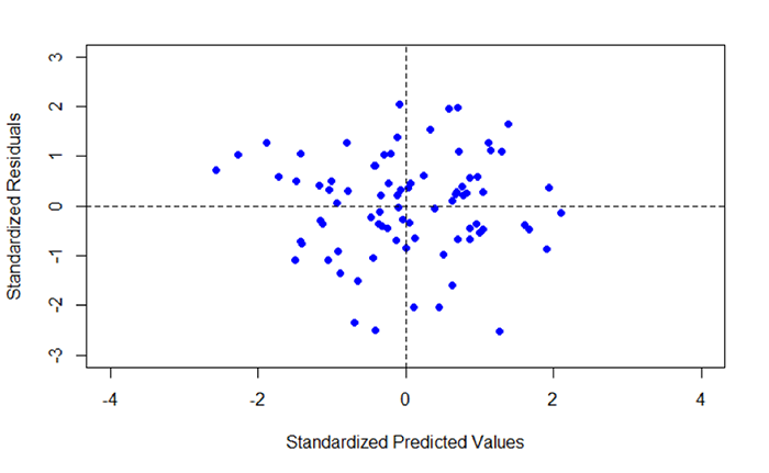
Fourth, create a scatterplot of the standardized residuals (y-axis) plotted against the standardized predicted value (x-axis).

>plot(Poverty_Regress$ZPR, Poverty_Regress$Std.Resids, pch = 19, col = "Blue", xlab = "Standardized Predicted Values", ylab = "Standardized Residuals", xlim = c(-4,4), ylim = c(-3,3))

Explaining some of the parameters in the plot command

• col is the color definition.
• xlim and ylim parameters control the numerical range shown on the x and y axes, respectively.
• bg is the background color. The scatterplot will have a grey background.
• pch is the plotting character used. In this case, the plotting character “19” is a solid fill circle whose fill is blue. For those of you with a more artistic background, here is a pdf of the color names used in r.

Figure 5.10 shows a scatterplot of the standardized predicted values (x-axis) plotted against the standardized residuals (y-axis). Note that there are two dashed lines drawn on the plot. Each dashed line is centered on 0. The dashed lines correspond to the mean of each standardized dataset. The other values represent standard deviations about the mean. Ideally, you would like to see a scatter of points that shows no trend. In other words, the scatter of points should not show an increase or decrease in data values going from + to - or - to + standard deviation. In Figure 5.10, we see a concentration that is more or less centered about the 0, 0 intersection, with the points forming a circular pattern.

Figure 5.10: A scatterplot of the standardized predicted values (x-axis) plotted against the standardized residuals (y-axis).

credit: Kessler 2019

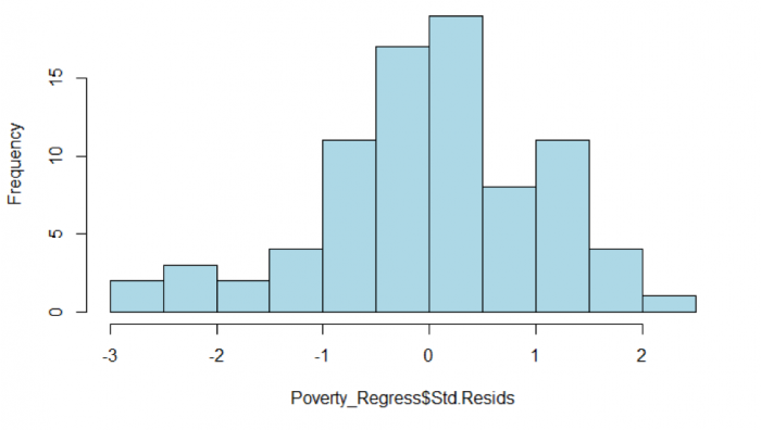
Fifth, create a histogram of the standardized residuals.

>hist(Poverty_Regress$Std.Resids, col = "Lightblue", main = "Histogram of Standardized Residuals")

In addition to examining the scatterplot, we can also view a histogram of the standardized residuals. By examining the distribution of the standardized residuals, we can see if the residuals appear to be normally distributed. This idea gets back to one of the assumptions of regression, which is that the errors of prediction are normally distributed (homoscedasticity). Looking at Figure 5.11, we see a distribution that appears to be fairly normally distributed.

Figure 5.11: A histogram of the standardized residuals.

credit: Kessler 2019

Assessing residuals for normality and homoscedasticity

It is important to test the standardized residuals for normality. For our test, we will use the Shapiro-Wilk normality test, which is available in the psych package.

>shapiro.test(Poverty_Regress$Std.Resids)

This command produced the following output.

Shapiro-Wilk normality test data:

Poverty_Regress$Std.Resids
W = 0.98025, p-value = 0.2381

Recall the hypothesis statement:
H₀: data are ≈ normal
H_A: data are ≈ not normal

The returned p-value is 0.2381. Using α = 0.05, the p-value is greater than 0.05, and thus we accept the null hypothesis that the standardized residuals are normal. This result helps to confirm that we have met the homoscedasticity assumption of regression.

Assessing the assumption of Independence: The Durbin-Watson Statistic

> durbinWatsonTest(Poverty_Regress$Std.Resids)

[1] 1.8058

In order to meet this assumption, we expect to see values close to 2. Values less than 1.0 or greater than 3.0 should be a warning that this assumption has not been met (Field, 2009). In this case, the Durbin-Watson statistic is 1.80, which suggests that we have met the condition of independence and no multicollinearity exists and the residuals are not autocorrelated.

Field, A.P. (2009). Discovering Statistics using SPSS: and Sex and Drugs and Rock ‘n’ Roll (3rd edition). London: Sage.

### Post-Regression Diagnostics
```{r}

# Compute the Predicted Values from the Regression
Poverty_Regress$Predicted <- predict(Poverty_Regress)

# Compute the Standardized Predicted Values from the Regression
Poverty_Regress$ZPR <- scale(Poverty_Regress$Predicted, center = TRUE, scale = TRUE)

# Compute the Standardized Residuals from the Regression
Poverty_Regress$Std.Resids <- rstandard(Poverty_Regress)

# Plot the Standardized Predicted Values and the Standardized Residuals
plot(Poverty_Regress$ZPR, Poverty_Regress$Std.Resids, pch = 19, col = "Blue", xlab = "Standardized Predicted Values", ylab = "Standardized Residuals", xlim = c(-4,4), ylim = c(-3,3))

# Divide the plot area into quadrate about the mean of x and y
abline(h=mean(Poverty_Regress$ZPR), lt=2)
abline(v=mean(Poverty_Regress$Std.Resids), lt=2)

# Plot a Histogram of Standardized Residuals
hist(Poverty_Regress$Std.Resids, col = "Lightblue", main = "Histogram of Standardized Residuals")

# Conduct a Normality Test on the Standardized Residuals
shapiro.test(Poverty_Regress$Std.Resids)

# Conduct a Durbin Watson Test on the Standardized Residuals
durbinWatsonTest(Poverty_Regress$Std.Resids)

```

Now you've walked through a regression analysis and learned to interpret its outputs. You'll be pleased to know that there is no formal project write-up required this week.