Review of Basic Statistical Analysis Methods for Analyzing Data - Part 2

Establishing Trends

Various statistical hypothesis tests have been developed for exploring whether there is something more interesting in one or more data sets than would be expected from the chance fluctuations Gaussian noise. The simplest of these tests is known as linear regression or ordinary least squares. We will not go into very much detail about the underlying statistical foundations of the approach, but if you are looking for a decent tutorial, you can find it on Wikipedia.  You can also find a discussion of linear regression in another PSU World Campus course: STAT 200.

The basic idea is that we test for an alternative hypothesis that posits a linear relationship between the independent variable (e.g., time, t in the past examples, but for purposes that will later become clear, we will call it x) and the dependent variable (i.e., the hypothetical temperature anomalies we have been looking at, but we will use the generic variable y).

The underlying statistical model for the data is:

where i ranges from 1 to N, a is the intercept of the linear relationship between y and x, b is the slope of that relationship, and ε is a random noise sequence. The simplest assumption is that ε is Gaussian white noise, but we will be forced to relax that assumption at times.

Linear regression determines the best fit values of a and b to the given data by minimizing the sum of the squared differences between the observations y and the values predicted by the linear model $\widehat{y}=a+bx$. The residuals are our estimate of the variation in the data that is not accounted for by the linear relationship, and are defined by

For simple linear regression, i.e., ordinary least squares, the estimates of a and b are readily obtained:

and

The parameter we are most interested in is b, since this is what determines whether or not there is a significant linear relationship between y and x.

The sampling uncertainty in b can also be readily obtained:

where std(ε) is standard deviation of ε and μ is the mean of x. A statistically significant trend amounts to the finding that b is significantly different from zero. The 95% confidence range for b is given by $b\pm 2{\sigma }_b$ . If this interval does not cross zero, then one can conclude that b is significantly different from zero. We can alternatively measure the significance in terms of the linear correlation coefficient, r , between the independent and dependent variables which is related to b through

r is readily calculated directly from the data:

where over-bar indicated the mean. Unlike b, which has dimensions (e.g., °C per year in the case where y is temperature and x is time), r is conveniently a dimensionless number whose absolute value is between 0 and 1. The larger the value of r (either positive or negative), the more significant is the trend. In fact, the square of r (r²) is a measure of the fraction of variation in the data that is accounted for by the trend.

We measure the significance of any detected trends in terms of a a p-value. The p-value is an estimate of the probability that we would wrongly reject the null hypothesis that there is no trend in the data in favor of the alternative hypothesis that there is a linear trend in the data — the signal that we are searching for in this case. Therefore, the smaller the p value, the less likely that you would observe as large a trend as is found in the data from random fluctuations alone. By convention, one often requires that p<0.05 to conclude that there is a significant trend (i.e., that only 5% of the time should such a trend have occurred from chance alone), but that is not a magic number.

The choice of p in statistical hypothesis testing represents a balance between the acceptable level of false positives vs. false negatives. In terms of our example, a false positive would be detecting a statistically significant trend, when, in fact, there is no trend; a false negative would be concluding that there is no statistically significant trend, when, in fact, there is a trend. A lower threshold (that is, higher p-value, e.g., p = 0.10) makes it more likely to detect a real but weak signal, but also more likely to falsely conclude that there is a real trend when there is not. Conversely, a higher threshold (that is, lower p-value, e.g., p = 0.01) makes false positives less likely, but also makes it less likely to detect a weak but real signal.

There are a few other important considerations. There are often two different alternative hypotheses that might be invoked. In this case, if there is a trend in the data, who is to say whether it should be positive (b > 0) or negative (b < 0)? In some cases, we might want only to know whether or not there is a trend, and we do not care what sign it has. We would then be invoking a two-sided hypothesis: is the slope b large enough in magnitude to conclude that it is significantly different from zero (whether positive or negative)? We would obtain a p-value based on the assumption of a two-sided hypothesis test. On the other hand, suppose we were testing the hypothesis that temperatures were warming due to increased greenhouse gas concentrations. In that case, we would reject a negative trend as being unphysical — inconsistent with our a priori understanding that increased greenhouse gas concentrations should lead to significant warming. In this case, we would be invoking a one-sided hypothesis. The results of a one-sided test will double the significance compared with the corresponding two-sided test, because we are throwing out as unphysical half of the random events (chance negative trends). So, if we obtain, for a given value of b (or r) a p-value of p = 0.1 for the two-sided test, then the p-value would be p = 0.05 for the corresponding one-sided test.

There is a nice online statistic calculator tool, courtesy of Vassar college, for obtaining a p-value (both one-sided and two-sided) given the linear correlation coefficient, r , and the length of the data series, N. There is still one catch, however. If the residual series ε of equation 6 contains autocorrelation, then we have to correct the degrees of freedom, N', which is less than the nominal number of data points, N. The correction can be made, at least approximately in many instances, using the lag-one autocorrelation coefficient. This is simply the linear correlation coefficient, r_1, between ε, and a carbon copy of ε lagged by one time step. In fact, r₁ provides an approximation to the parameter ρ introduced in equation 2. If r₁ is found to be positive and statistically significant (this can be checked using the online link provided above), then we can conclude that there is a statistically significant level of autocorrelation in our residuals, which must be corrected for. For a series of length N = 100, using a one-sided significant criterion of p = 0.05, we would need r₁ > 0.17 to conclude that there is significant autocorrelation in our residuals.

Fortunately, the fix is very simple. If we find a positive and statistically significant value of r₁, then we can use the same significance criterion for our trend analysis described earlier, except we have to evaluate the significance of the value of r for our linear regression analysis (not to be confused with the autocorrelation of residuals r₁) using a reduced, effective degrees of freedom N', rather than the nominal sample size N. Moreover, N' is none other than the N' given earlier in equation 3 where we equate $$\rho =r_1$$

That's about it for ordinary least squares (OLS), the main statistical tool we will use in this course. Later, we will encounter the more complicated case where there may be multiple independent variables. For the time being, however, let us consider the problem of trend analysis, returning to the synthetic data series discussed earlier. We will continue to imagine that the dependent variable (y) is temperature T in °C and the independent variable (x) is time t in years.

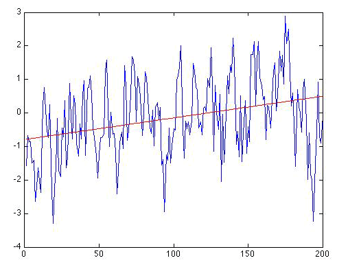
First, let us calculate the trend in the original Gaussian white noise series of length N = 200 shown in Figure 2.12(1). The linear trend is shown below:

Figure 2.12(6): N=200 years of Gaussian White Noise with linear trend shown.

Credit: Michael Mann

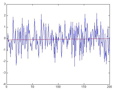
The trend line is given by: $\widehat{T}=0.0006\cdot t-0.1140$, and the regression gives r = 0.0332. So there is an apparent positive warming trend of 0.0006 °C per year, or alternatively, 0.06 °C per century. Is that statistically significant? It does not sound very impressive, does it? And that r looks pretty small! But let us be rigorous about this. We have N = 200, and if we use the online calculator link provided above, we get a p-value of 0.64 for the (default) two-sided hypothesis. That is huge, implying that we would be foolish in this case to reject the null hypothesis of no trend. But, you might say, we were looking for warming, so we should use a one-sided hypothesis. That halves the p-value to 0.32. But that is still a far cry from even the least stringent (e.g., p = 0.10) thresholds for significance. It is clear that there is no reason to reject the null hypothesis that this is a random time series with no real trend.

Next, let us consider the red noise series of length N = 200 shown earlier in Figure 2.12(2).

Figure 2.12(7). N=200 years of Gaussian 'red noise' with ρ=0.6 with linear trend shown.

Credit: Michael Mann

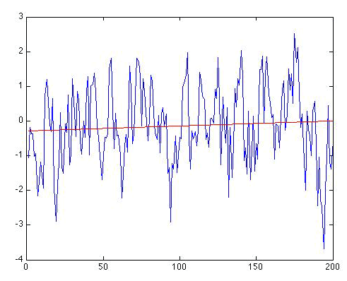
As it happens, the trend this time appears nominally greater. The trend line is now given by: $\widehat{T}=0.0014\cdot t-0.2875$, and the regression gives r = 0.0742. So, there is an apparent positive warming trend of 0.14 degrees C per century. That might not seem entirely negligible. And for N = 200 and using a one-sided hypothesis test, r = 0.0742 is statistically significant at the p = 0.148 level according to the online calculator. That does not breach the typical threshold for significance, but it does suggest a pretty high likelihood (15% chance) that we would err by not rejecting the null hypothesis. At this point, you might be puzzled. After all, we did not put any trend into this series! It is simply a random realization of a red noise process.

The problem is that our residuals are not uncorrelated. They are red noise. In fact, the residuals looks a lot like the original series itself:

Figure 2.12(8). Residuals from linear regression with N=200 years of Gaussian 'red noise' with ρ=0.6

Credit: Michael Mann

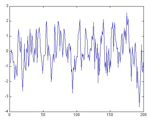
This is hardly coincidental; after all, the trend only accounts for $r^2={0.0742}^2=0.0055$, i.e., only about half a percent, of the variation in the data. So 99.5% of the variation in the data is still left behind in the residuals. If we calculate the lag-one autocorrelation for the residual series, we get r₁ = 0.54. That is, again not coincidentally, very close to the value of ρ = 0.6 we know that we used in generating this series in the first place.

How do we determine if this autocorrelation coefficient is statistically significant? Well, we can treat it like it were a correlation coefficient. The only catch is that we have to use N-1 in place of N, because there are only N-1 values in the series when we offset it by one time step to form the lagged series required to estimate a lag-one autocorrelation.

If we use the online link and calculate the statistical significance of r₁ = 0.54 with N-1 = 199, we find that it is statistically significant at p < 0.001. So, clearly, we cannot ignore it. We have to take it into account.

So, in fact, we have to treat the correlation from the regression r = 0.074 as if it has $N\text{'}=\left(1-0.54\right)/\left(1+0.54\right)200=0.30\left(200\right)=59.9$ ≈ 60 degrees of freedom, rather than the nominal N = 200 degrees of freedom. Using the interactive online calculator, and replacing N = 200 with the value N' = 60, we now find that a correlation of r = 0.074 is only significant at the p = 0.57 (p = 0.29) for a two-sided (one-sided) test, hardly a level of significance that would cause us to seriously call into doubt the null hypothesis.

At this point, you might be getting a bit exasperated. When, if ever, can we conclude there is a trend? Well, why don't we now consider the case where we know we added a real trend in with the noise, i.e., the example of Figure 2.12(5) where we added a trend of 0.5°C/century to the Gaussian white noise. If we apply our linear regression machinery to this example, we do detect a notable trend:

Figure 2.12(9). N=200 years of Gaussian white noise with added linear trend of 0.5 degrees/century; the red line shows trend recovered by the linear regression.

Credit: Michael Mann

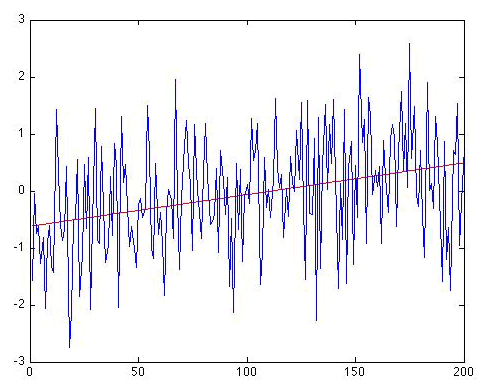
Now, that's a trend - your eye isn't fooling you. The trend line is given by: $\widehat{T}=0.0056\cdot t-0.619$. So there is an apparent positive warming trend of 0.56 °C per century (the 95% uncertainty range that we get for b, i.e., the range b±2 σ_b, gives a slope anywhere between 0.32 and 0.79 °C per century, which of course includes the true trend (0.5 °C/century) that we know we originally put in to the series!). The regression gives r = 0.320. For N = 200 and using a one-sided hypothesis test, r = 0.320 is statistically significant at p<0.001 level. And if we calculate the autocorrelation in the residuals, we actually get a small negative value ($r_1=-0.095$), so autocorrelation of the residuals is not an issue.

Finally, let's look at what happens when the same trend (0.5 °C/century) is added to the random red noise series of Figure 2.12(2), rather than the white noise series of Figure 2.12(1). What result does the regression analysis give now?

Figure 2.12(10). N=200 years of Gaussian red noise with ρ=0.6 and added linear trend of 0.5 degrees/century; the red line shows trend recovered by the linear regression.

Credit: Michael Mann

We still recover a similar trend, although it's a bit too large. We know that the true trend is 0.5 degrees/century, but the regression gives: $\widehat{T}=0.0064\cdot t-0.793$. So, there is an apparent positive warming trend of 0.64 °C per century. The nominal 95% uncertainty range that we get for b is 0.37 to 0.92 °C per century, which again includes the true trend (0.5 degrees C/century). The regression gives r = 0.315. For N = 200 and using a one-sided hypothesis test, r = 0.315 is statistically significant at the p < 0.001. So, are we done?

Not quite. This time, it is obvious that the residuals will have autocorrelation, and indeed we have that r₁ = 0.539, statistically significant at p < 0.001. So, we will have to use the reduced degrees of freedom N'. We have already calculated N' earlier for ρ = 0.54, and it is roughly N' = 60. Using the online calculator, we now find that the one-sided p = 0.007, i.e., roughly p = 0.01, which corresponds to a 99% significance level. So, the trend is still found to be statistically significant, but the significance is no longer at the astronomical level it was when the residuals were uncorrelated white noise. The effect of the "redness" of the noise has been to make the trend less statistically significant because it is much easier for red noise to have produced a spurious apparent trend from random chance alone. The 95% confidence interval for b also needs to be adjusted to take into account the autocorrelation, though just how to do that is beyond the scope of this course.

Often, residuals have so much additional structure — what is sometimes referred to as heteroscedasticity (how's that for a mouthful?) — that the assumption of simple autocorrelation is itself not adequate. In this case, the basic assumptions of linear regression are called into question and any results regarding trend estimates, statistical significance, etc., are suspect. In this case, more sophisticated methods that are beyond the scope of this course are required.

Now, let us look at some real temperature data! We will use our very own custom online Linear Regression Tool written for this course. The demonstration how to use this tool has been recorded in three parts below. Here is a link to the online statistical calculator tool mentioned in the videos below.

In addition, there is a written tutorial for the tool and these data available at these links: Part 1, Part 2.

Video: Custom Linear Regression Tool - Part 1 (3:16)

Video: Custom Linear Regression Tool - Part 2 (1:03)

Video: Custom Linear Regression Tool - Part 3 (1:53)

You can play around with the temperature data set used in this example using the Linear Regression Tool