Prioritize...
After completing this section, you will have executed your first script in R-Studio. NOTE: If you have not completed the lessons in "swirl", I suggest you do that now.
Read...
In most of the tutorials that you have explored (especially the "swirl" examples), you entered every command in the console window. This approach is occasionally useful when we want to query an previously-loaded dataset, or when we want test a command or procedure. However, most of the time, we are going to place all of our commands in an R-script file (mainly because we don't want to have to retype every command each time we want to perform some sort of calculation). Secondly, saving everything in script files means that we can retrieve processes created for previous tasks -- to be either reused or modified to fit your needs.
A word of advice!
You will find that we will constantly be building on (or reusing) snippets of R-code. You do not want to be reinventing the wheel every time. Therefore, I suggest keeping an organized directory structure of R-script files (for example, by course and lesson perhaps) that have explanatory filenames (e.g., basic_scatterplot.R; not, my_code.R). Furthermore, I suggest that you have a few lines of comments at the beginning of each script that explains what the code does (and allows for easy searching). This will help tremendously if you need to find a particular piece of code sometime in the future -- and you will, trust me. You might also consider storing this directory in the cloud to both keep it safe and also allow access from various computers. There are several free cloud services that give you plenty of storage space.
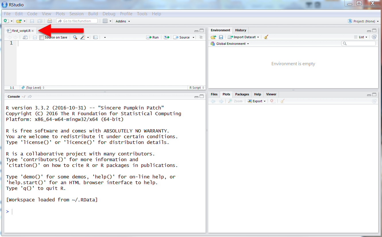
Once you've set up a place to put your R-scripts, let's create your first one. Open up R-Studio and select "File > New File > R script". Next, select "File > Save". Save the script in the folder structure you just created and name this script "first_script.R". Notice that after you save it, the name appears in the tab. Now, copy and paste the code below into your new script (remember to save it afterwards).
# assign some variables
x <- c(1:25)
y <- x^2
z <- seq(1, 21, by=2)
rand_nums <- runif(100, min=-1, max=1)
my_colors <- c("red", "blue", "green")
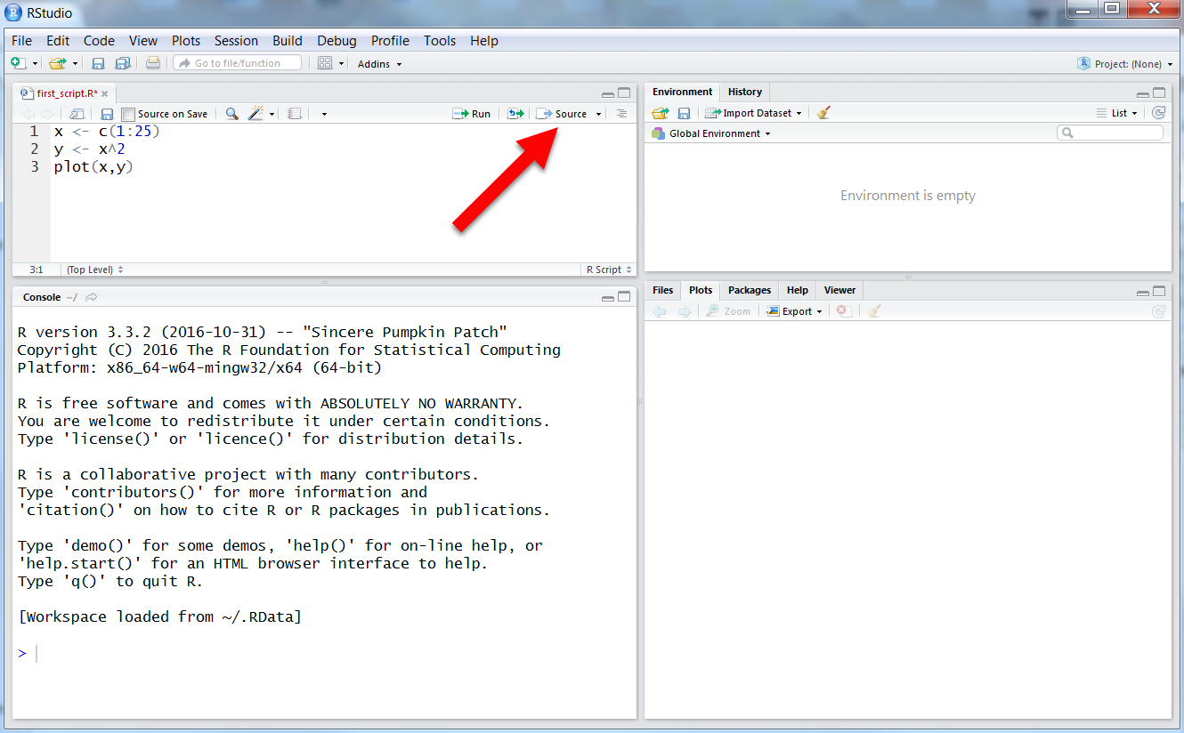
I know, since you've completed the swirl tutorials, you are familiar with the commands above. If you can't quite remember, recall you can always type ?<command> in the console window to find out more about a particular command. Give it a try on the command runif() to learn more about it (Of course, you could also just Google: "R runif" as well. Try it!). To execute this bit of code, click on the "Source" button in the upper-right corner of the script window. After sourcing the script, you should notice that in the upper-right panel you should see a list of values for x, y, z, rand_nums, and my_colors. You'll find the information in the environment panel helpful when checking to see if your code is working like you'd expect. Notice that the panel shows you what variables are currently being stored by R, how many elements they contain, what "type" of data (numbers, characters, integers, etc.) each variable contains, along with some values.
Return to the script and focus your attention on variable "y". In the assignment statement, we defined "y" as the square of variable "x". In many programming languages, "x" would be considered an array. Therefore, to perform calculations on "x" you would have to loop through each value of the array sequentially. Remember however, that R performs what we refer to as Vector Arithmetic. When you add two variables (say, x + y), R interprets this as adding the vector "x" to the vector "y", term by term. R's approach to variable arithmetic saves us a tremendous amount of time because we don't need to loop over all the values for every computation we need to perform. Instead, we simply tell R what to do, and the program figures out how to do it. (Review Lesson 4 of the "swirl" tutorial for more information on R vector variables.)
Importing Data From a File
Now, you might have guessed that we could never enter the vast amounts of data we need into R using assignment statements like we just did above. So, let’s explore how to import data into R from a file. Start by saving this comma delimited file, UNV_maxmin_td_2014.csv, to your local machine by right-clicking the link and selecting “Save Link As…”. Save your file to the same folder that contains the script you created above.
Add the following line of code to your R-script file that you have open:
mydata <- read.csv("UNV_maxmin_td_2014.csv")
Now, source the file. You probably received an error telling you that R couldn’t find the file. This is because we only specified the filename the we want to open, not the entire file path. You can specify the entire path like this:
mydata <- read.csv("C:/Files/Meteo810/Lesson3/R_code/UNV_maxmin_td_2014.csv")
Your path will be different, of course, but you get the idea.
Using the full path name can be useful in some instances (you can even specify HTTP or FTP addresses). However, most of the time, I suspect that you will find typing all the path names tiring. Never fear! You can just tell R to use a default "working" directory whenever it looks for files. You can find out what the current working directory is by typing: getwd() in the console. To change the working directory, you use the command setwd(<directory>). You can use this command either in the console or right at the top of your script. For example, modify your script by adding a line containing setwd():
setwd("C:/Files/Meteo810/Lesson3/R_code/")
mydata <- read.csv("UNV_maxmin_td_2014.csv")
Notice above that we use the backslash (like an Internet address) even if we have the Windows OS (which uses the "\" to designate file paths). If you are uncomfortable figuring out the path to a particular folder, R-Studio offers an even easier way to set the working directory. You can set the working directory by selecting (Session->Set Working Directory->Choose Directory…) from the main menu of R-Studio. Once you point R-Studio to the proper directory, try re-sourcing the original code (with just the filename). If you don't get an error in the console window, you did it correctly.
Before moving on...
Take a moment to explore the options available for the read.csv() command. Type ?read.csv() into the R-Studio console or Google "R read.csv". Here's some documentation describing read.csv() and its sister functions. Note the host of arguments that you can pass the function. You can skip rows, rename columns, and recast the datatypes, just to name a few.
Now that you have loaded the data file, examine the Environment tab in the upper-right panel. You should see a new variable called “mydata” located under a the new heading "Data" instead of "Values". This variable is referred to as a dataframe. Dataframes are used for storing tables of values in lists of equal-sized vectors. In R-studio, you can expand the dataframe by clicking the little blue arrow directly in front of the name. This gives you information about each variable in the dataframe. For example, you’ll note that it contains three variables: date, max_dwpf, and min_dwpf. You can also view the data in table format by clicking on the grid icon located to the right of its name in the Environment tab. This gives you a spreadsheet view of the dataframe where you can examine, sort, and filter the data (but you cannot edit it).
Now that we've loaded some data, let's look at how we might interact with it. Read on.