Custom Plots

Read...

We have looked at many different types of plots so far in this lesson. But what if we want a plot that is not included in the standard libraries? A wind rose for example.

Think of a wind rose as a circular histogram of wind directions and speeds. These graphics are used by those interested in wind climatology. So, how might we get R to generate a wind rose? Certainly, given R’s powerful programming language, we could figure out the commands necessary to generate the plot that we want. However, there’s a better way. We can look for someone who has already done the work for us. Because R is open-source, people from all over the world are actively writing and contributing new functions that everyone can use. These new functions are grouped together into packages found on the R-project website.

With a little searching, I discovered a package named “openair” which (among other things) plots wind roses. If you look at the user’s manual, you’ll discover all sorts of functions that deal with the analysis and display of air pollution data. At this time, I’m only interested in accessing the wind rose function.

First, I need to download and install the package. Here, R-studio is of great help. In the lower-right panel, click on the “Packages” tab. This displays all of the currently downloaded packages. Click on the “install” button, and in the dialog box that appears, type the package’s name: “openair” in the space available (leave everything else as default). You can also have the script check for and install the package by adding code such as lines 7-8 below.

Open a new R-script file and enter the following code (but don't source the file yet):

# you can find this code in: wind_rose.R

# This code plots the a wind rose using the package "openair"

# check to see if openair has been installed
# if not, install it
if (!require("openair")) {
  install.packages("openair") }

# connect to the openair package
library(openair)

# Read in the RAW 5-minute ASOS file...
wind_data <- read.fwf("64010KPHL201401.dat", 
                       widths=c(-28, 17, -21, 3,2),
                       header=FALSE, 
                       col.names = c("date","wd","ws"))

# Convert the fields to the proper data types
# Packages often require strict adherence to data rules
wind_data$date <- as.POSIXct((strptime(wind_data$date, format = "%m/%d/%y %H:%M:%S")))
wind_data$wd<-as.numeric(as.character(wind_data$wd))
wind_data$ws<-as.numeric(as.character(wind_data$ws))

# plot the wind rose
windRose(wind_data, angle=10,
         paddle=F, breaks=c(0,5,10,15,20,25), seg=0.65,
         offset=5, main = "Winds at KPHL, January 2014",
         key=list(footer="knots", height=1)
)

Let's break it down.... First, we must tell R that we are including functions that are not part of its core set of commands.  The line, library(openair) tells R to recognize all of the functions included in the package openair. If you don’t include this line, you will get an error when you try to use the windRose command which is only defined as part of the openair library. Next, we read the raw ASOS file of 5-minute averaged data for the Philadelphia International Airport during January 2014 (to download the file, right-click -> Save As... on the link).  If you want to grab your own data, you can get it from the ASOS NCDC page (click on the 5-minute data link).  Take a look at the file... it's a mess of numbers. After reviewing the "td6401b.txt" documentation found in the data directory, I decided to read the file into R using read.fwf() which reads in fixed-width files. Pay particular attention to the widths fields. I start out by ignoring the first 28 characters, then I read in the next 17, ignore 21 more, then read in 3 characters and 2 characters.  I name the columns that I kept as "date", "wd", and "ws" (the "wd" and "ws" are required column names for the windrose command).  Next, I needed to convert the columns into their proper data type (there's that nebulous type called a "factor" again).

Finally, let's look at the windRose command. How did I know how to use it? Remember that you can always type “?command” in the console window to see how a command is used. Or better yet, click on the packages tab (that you just used to install the openair package), find the “openair” package in the list, and click on it. Now you are given a listing of all the functions contained in the package. Scroll to the bottom and select the windRose function. Now you can see the usage and all the possible parameters that can be included.

You're welcome to play around with various settings to see how they affect the plot. I did, however, want to point out a fact about the input data. It's very important to make sure that your data match what the functions are expecting.  In the case of windRose, the function requires a data frame that has columns with names "ws" (for speed) and "wd" (for direction).  In the interest of full disclosure, I note that the documentation says that you can specify by name which columns are speed and direction, but I have found if you deviate from the "ws" and "wd" names, the function can behave unpredictably.

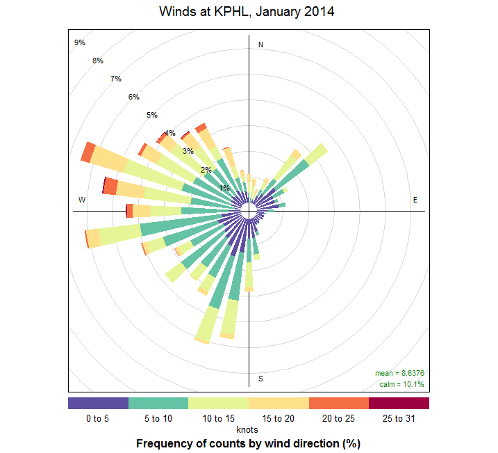
Finally, if you haven't already, source the file and generate the plot (seen below).  We can see a few interesting trends.  First, the winds during this time appear to come from two general quadrants: southwest, and northwest. The winds from the southwest tend to be lighter -- less than 10 knots. Northwest winds have higher observed wind speeds. We can see these trends if we examine the histograms of wind speed for NW versus SW directions. Since this is January, I suspect the strong NW winds follow in the wake of strong cold fronts.

A wind rose for Philadelphia International Airport. Data represent the occurrence of wind speed and direction during January 2014.  Colors and lengths of bars represent the fraction of time that wind was observed blowing from each direction at a given speed.

Credit: D. Babb

Throughout this course, we will be using packages built by others. You will discover that doing so is extremely convenient in retrieving and navigating large data sets.  Some institutions like NOAA or NCDC even offer their own packages specially designed to interface with their own data. This saves us a great deal of time and effort. If you find you want to do something unique (or even find a better set of plotting tools) look first for a package to do the job.