3.2.2: Porosity from Well Logs

The most common method of determining porosity is with Well Logs. Well logs are tools sent down the wellbore during the drilling process which measure different reservoir properties of interest to geologists and engineers. Due to the expense of obtaining core samples, typically only a few wells are cored. The wells that do get cored are usually wells early in the life of the reservoir (appraisal wells) and key wells throughout the reservoir. On the other hand, well logs are routinely run in wells, if only to identify the depths of the productive intervals. The three open-hole logs used to evaluate porosity are:

• The sonic log
• The density log
• The neutron log

While none of these logs measures porosity directly, the porosity can be calculated based on theoretical or empirical considerations. The measurements obtained from these logs are not only dependent on the porosity but are also dependent on other rock properties such as:

• Lithology (rock type: sandstone, limestone, shale, etc.)
• The fluids occupying the pore spaces
• The wellbore environment (type of drilling fluid, hole size)
• The geometry of the pores

Since many variables may impact the log readings, corrections need to be applied to the log interpretations and the three logs are typically evaluated together to determine the best estimate of the porosity of rock formations. The log evaluations are also calibrated against core porosity in wells where both core and logs are available.

The Sonic Log measures the acoustic transit time, Δt, of a compressional sound wave traveling through the porous formation. The logging tool consists of one or more transmitters and a series of receivers. The transmitters act as sources of the acoustic signals which are detected by the receivers. The time required for the signal to travel through one foot of the rock formation is the acoustic transit time, Δt. The acoustic travel time, then, is the reciprocal of the sonic velocity through the formation. The units of Δt are micro-seconds/ft (μsec/ft) or millionths of a second per foot.

There are several ways to interpret the sonic log measurements. One of the most common interpretation formulae is the Wyllie Time-Average Equation:

Where:

• ϕ_sl is the porosity from the sonic log (log measurement) , fraction
• Δt_sl is value of the acoustic transit time measured by the sonic log, μsec/ft
• Δt_ma is value of the acoustic transit time of the rock matrix measured in the laboratory, μsec/ft
• Δt_f is value of the acoustic transit time saturating fluid measured in the laboratory, μsec/ft

The presence of hydrocarbons in the reservoir rock results in an over prediction of porosity measured by the sonic log and some corrections may be required. These corrections take the form:

or,

Table 3.03 has typical values of the acoustic transit time for different reservoir formations and commonly encountered reservoir fluids.

Table 3.03: Typical Acoustic Transit Times for Sonic Log Interpretation

Heading1	Δtma (μsec/ft) Range	Δtma (μsec/ft) Commonly Used	Δtf (μsec/ft) Range	Δtf (μsec/ft) Commonly Used
Sandstone	55.5 – 51.0	55.5 or 51.0	—	—
Limestone	47.8 – 43.5	47.5	—	—
Dolomite	43.5	43.5	—	—
Anhydrite	50.0	50.0	—	—
Salt Formation	66.7	67.0	—	—
Fresh Water Based Drilling Fluid	—	—	189.0	189.0
Salt Water Based Drilling Fluid	—	—	185.0	185.0
Gas	—	—	920.0	920.0
Oil	—	—	230.0	230.0
Casing (Iron)	—	—	57.0	57.0

Other empirically based equations exit for sonic log interpretation. One form of an alternative equation is:

In this equation, the value of C is in the range of 0.625 to 0.700 and is determined by calibrating the equation to known porosity, such as, to core data when a well is both cored and logged. In Equation 3.12 and Equation 3.13, ϕ_sonic is the final interpreted porosity from the sonic log.

The _{Density Log} measures the electron density ρ_e, of the formation (the electron density is the number of electrons per unit volume). The density logging tool emits gamma rays from a chemical source which interact with the electrons of elements in the formation. Detectors in the tool count the returning gamma rays. These returning gamma rays are related to the election density of the elements in the formation.

The electron density is proportional to the bulk density, ρ_b, of the formation (the bulk density is the density of the fluid-filled rock in grams per unit volume). For a molecular substance, this proportionality is:

Where:

• ${\rho }_e$ is the electron density of the formation, electrons/cc
• ${\rho }_b$ is the bulk density of the formation, gm/cc
• ΣZ is the sum of the atomic numbers making up the molecule, electrons/molecule
• MW is the molecular weight, gm/molecule

Table 3.04 contains the term in the parenthesis for common substances related to oil and gas production.

Table 3.04: Properties for Density Log Interpretation

Compound	Chemical Formula	Actual Density, ${\rho }_b$ (gm/cc)	$\left(\frac{\text{2}{\displaystyle \sum \text{z}}}{\text{MW}}\right)$ (electrons/gm)	Electron Density, ${\rho }_e$ (electrons/cc)	Log Reading, Apparent ${\rho }_{ba}$ (gm/cc)
Quartz	SiO2	2.654	0.9985	2.650	2.648
Calcite	CaCO3	2.710	0.9991	2.708	2.710
Dolomite	CaCO3MgCO3	2.870	0.9977	2.863	2.876
Anhydrite	CaSO4	2.960	0.9990	2.957	2.977
Sylvite	KCl	1.984	0.9657	1.916	1.863
Halite	NaCl	2.165	0.9581	2.074	2.032
Gypsum	CaSO42H2O	2.320	1.0222	2.372	2.351
Anthracite Coal	---	1.400 - 1.800	1.0200	1.442 – 1.852	1.355 – 1.796
Bituminous Coal	---	1.200 - 1.500	1.0600	1.227 – 1.590	1.173 – 1.514
Fresh Water	H2O	1.000	1.1101	1.110	1.000
Brine (200,000 ppm)	---	1.146	1.0797	1.237	1.135
Oil	N(CH2)	0.850	1.1407	0.970	0.850
Methane	CH4	${\rho }_{methane}$	1.2470	1.247 ${\rho }_{methane}$	1.335 ${\rho }_{methane}$ - 0.1883
Gas	---	${\rho }_{gas}$	1.2380	1.238 ${\rho }_{gas}$	1.238 ${\rho }_{gas}$ - 0.1883

One important observation from this table is that the column containing the group in parenthesis in Equation 3.14, $\left(\frac{\text{2}{\displaystyle \sum \text{z}}}{\text{MW}}\right)$ , is approximately 1.0. Since this term is close to unity, the electron density is a very close approximation to the bulk density, as also seen in Table 3.03. The logging tool is calibrated by running it against a limestone formation containing fresh water. With this calibration, the Log Reading, Apparent ρ_ba (last column in Table 3.03) is:

For some substances, such as liquid-filled sandstones, limestones, and dolomites, ρba can be used directly as ρ_b. For other substances, such as sylvite, rock salt, gypsum, anhydrite, coal, and gas bearing formations, further corrections are required. These additional corrections are beyond the scope of this course. Once the bulk density is determined, the porosity can be estimated by:

Where:

• ϕ_density is the final interpreted porosity from the density log, fraction
• ρ_ma is the matrix density (from the Actual Density, ρ_b, Column in Table 3.03), gm/cc
• ρ_b is bulk density from density log (Equation 3.15), gm/cc
• ρ_f is the density of the fluid measured in the laboratory, gm/cc

The Neutron Log measures the amount of hydrogen in the formation being logged. Since the amount of hydrogen per unit volume is approximately the same for oil and water, the neutron log measures the Liquid Filled Porosity (the porosity excluding the Gas-Filled Porosity). The neutron logging tool emits neutrons from a chemical source which collide with nuclei of elements in the formation. The element in the formation with the mass closest to a neutron is hydrogen. Due to the parity in mass, the neutron in a neutron-hydrogen collision loses approximately half of its energy. With enough collisions, the neutron eventually loses enough energy and is absorbed by the hydrogen nucleus and a gamma ray is emitted. The neutron logging tool measures these emitted gamma rays. Note, other hydrogen atoms may be present in clays in the rock, or in the rock itself and corrections for these other hydrogen atoms are required.

Interpretation of the neutron log is performed by first calibrating the logging tool to specific well and formation conditions. Interpretation charts supplied by the logging company are used to interpret the log for deviations from these calibration conditions. The interpretation of the neutron log for ϕ_neutron is beyond the scope of this course.

As mentioned throughout the discussion on porosity logging, due to the various wellbore and formation conditions encountered during the logging operations (i.e., real conditions, as opposed to laboratory conditions) many corrections may be required to get a good interpretation from the different well logs. In addition, the logs are typically evaluated together to aid in the interpretation. Finally, if core data are available from a well, then the core derived porosity is used to calibrate the logging tools.

Rock (Pore-Volume) Compressibility

In addition to the porosity and its relation to pore-volume, reservoir engineers are also interested in how the pore-volume behaves (increases or decreases) with increases or decreases in pore-pressure. The industry standard relationship for change in pore-volume is based on the isothermal pore-volume compressibility, c_PV.

The isothermal pore-volume compressibility is always positive and is defined as:

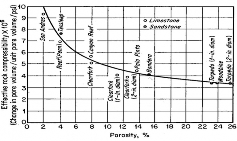
The units of compressibility are 1/psi. Equation 3.17 implies that as pressure increases the pore-volume increases. Hall ^[4] correlated the effective rock compressibility as a function of porosity which is shown in Figure 3.04.

For a constant bulk volume and compressibility, we can separate variables in Equation 3.17 and integrate to arrive at the following relationship between pore-volume (or porosity) and pore pressure:

or,

Where ϕ_ref is a reference porosity measured at reference pressure, p_ref. After some manipulation:

To further simplify this relationship, if we assume a small pore-volume compressibility (as shown in Figure 3.03, we are typically dealing with rock compressibilities on the order of 10^-6 1/psi) and apply a Taylor Series expansion to the exponential function (truncated after one term), we obtain:

The rock compressibility determination is performed in the laboratory on core samples. The rock compressibility is an expensive test to run and is not part of the Routine Core Analysis. It must be specifically requested as part of any Special Core Analysis, or SCAL, testing performed on the core sample.

Rock Permeability

The permeability of a porous medium is a measure of the ease (or difficulty) in which a fluid can flow through the pores of the medium. Permeability is a property of the porous medium which in our case is the reservoir rock. The unit of permeability is the Darcy, or D, named after the French engineer Henri Darcy who investigated the flow of water through filter beds in the city of Dijon in the mid-1800s. The unit of Darcy has the dimensions of length-squared. One significant contribution from Darcy’s work (among many), is Darcy’s Law, which was published in 1856 and forms one of the foundations of porous media flow:

Where:

• q_w is the flow rate of water, cc/sec
• k is the permeability of the medium, Darcy
• A is cross-sectional area, cm²
• l is the length in the direction of flow, ft (x, y, or z in Cartesian coordinates)
• $\frac{\partial p}{\partial l}$ is the pressure gradient, atm/cm

The unit of the Darcy is defined as the permeability, k, required to allow a flow rate, q_w, of one cc of water per second through a medium with a cross-sectional area, A, of one cm², with an applied pressure gradient, Δp/ΔL, of one atm/cm. As it turns out, the Darcy as a unit is too large for most field applications. In reservoir engineering we typically work with the millidarcy, md, which is one one-thousandth of a Darcy:

$$\text{1 D = 1,000 md}$$

Henri Poiseuille later generalized Darcy’s Law to fluids other than water by noting that the flow rate was inversely proportional to the dynamic viscosity, μ_f, of the fluid flowing through the porous medium. The unit of dynamic viscosity, the poise, is named after Poiseuille and is a property of the fluid. Again, as it turns out, the poise as a unit is also too large for most field applications. In reservoir engineering we typically work with the centipoise, cp, which is one one-hundredth of a poise:

$$\text{1 poise = 100 cp}$$

The generalized form of Darcy’s Law for any single-phase fluid which incorporates the fluid viscosity is:

Darcy’s Law has several important assumptions associated with it. These include:

• A rigid porous medium (incompressible medium with no transport of rock grains, e.g. fines movement
• An incompressible, homogeneous, Newtonian fluid that fully saturates (single-phase) the porous medium
• Steady-state, isothermal, and laminar (low Reynolds number) flow conditions
• No interactions between the porous medium and the fluid flowing through it
• A no-slip interface between the porous medium and the fluid flowing through it (zero velocity boundary condition at the rock-fluid interface)

The form of Darcy’s Law discussed so far uses the SI unit system. For oilfield units, we have:

Where:

• q_f is the flow rate of the saturating fluid, bbl/day
• 0.001127 is a unit conversion constant
• k is the absolute permeability of the medium, md
• A is cross-sectional area, ft²
• $\frac{\partial p}{\partial l}$ is the pressure gradient, psi/ft

Measurement of the permeability can be done through laboratory or field measurements. In the laboratory, a core sample of known dimensions (A and ΔL) is cleaned and placed into a fluid-tight core holder. A fluid of known viscosity (typically air) is allowed to flow through the core at a metered flow rate. Darcy’s Law is then used to calculate the permeability of the core sample.

In the field, permeability is measured with a Well Test using Pressure Transient Analysis. Under certain conditions, the production rate(s) (can be a zero-production rate) results in well pressures that honor known solutions to the Diffusivity (or Well Test) Equation. When the well test results are compared to the solutions to the diffusivity equation, the permeability of the formation can be estimated.

One common well test is a Pressure Build-Up Test. In a pressure build-up test, the well is produced at a stable (constant) rate, q_p, for a production time of t_p. The well is then shut in and the pressure is monitored during the shut-in period Δt; where Δt is measured from the beginning of the well is shut-in. The well test is called a build-up test because when the well is shut in, the pressures increase with increasing Δt. One analysis tool for the pressure build-up test is the Horner Plot. A typical Horner plot is shown in Figure 3.05.

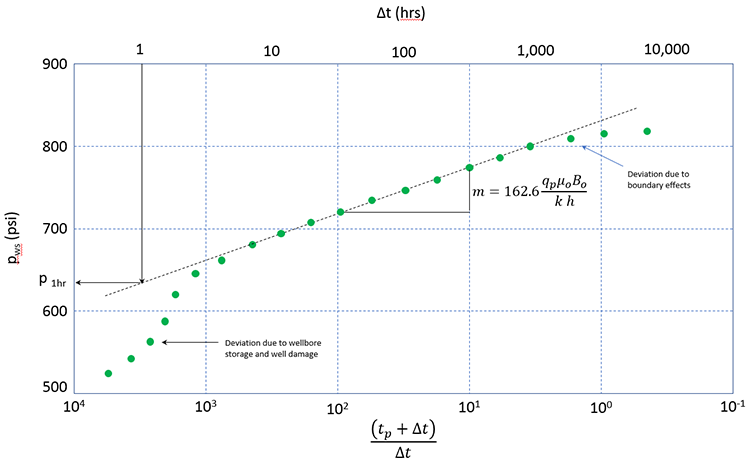
In this plot shown in Figure 3.05, p_ws are the shut-in well pressures measured during the well test, t_p and Δt are times in hours (Δt measured from the time that the well is shut-in), q_p is the stabilized production rate during the production period prior to well shut-in in STB/day, μ_o is the oil viscosity in cp, B_o is the Formation Volume Factor in bbl/STB, k is the permeability in md, and h is the reservoir thickness in ft.

In a Horner Plot, the function $\frac{\left(t_p+\Delta t\right)}{\Delta t}\left(bottomx-axis\right)$ , decreases as $\Delta t\left(topx-axis\right)$ increases. As can be seen in this figure, the slope of the Horner Plot is related to the permeability of the reservoir near the well. If the shut-in pressures, p_ws, are measured and the slope calculated, then the permeability can be determined if all the other parameters in the definition of the slope are known.

In semi-logarithmic plots (plots with one conventional axis and one logarithmic axis), such as that in Figure 3.05, the slope is normally taken over one logarithmic cycle. That is:

While there is no universal correlation between permeability, field measurements suggest that as the porosity of a formation increases, the permeability of the formation also increases. This behavior is captured in a permeability-porosity cross-plot. One such example of a permeability-porosity cross plot is illustrated in Figure 3.06.

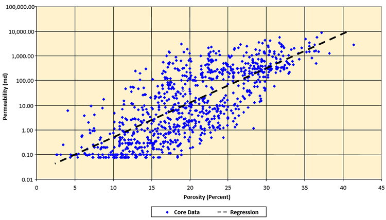
A permeability-porosity cross-plot is a field dependent transform that relates core derived permeability to core derived porosity. Note that the permeability-porosity transform shown in Figure 3.06 is plotted on a semi-logarithmic plot with the permeability plotted on the logarithmic scale. Also note that in the middle of the plot (ϕ = 20 percent) there is an approximate four order of magnitude error bar in the permeability data. This is typical for a permeability-porosity transform. While the results from these transforms may be crude, they are often the only source of permeability data when building complex models of oil or gas reservoirs. Note, geologists have developed methods for capturing this scatter into their models in the form of Scatter Plots, but the development of such plots is beyond the scope of this course.

The permeability in the presence of a single-phase fluid is called the absolute permeability. Since we will be dealing with multi-phase flow, we will need to discuss extensions to Darcy’s which allow for more than one phase. We will do this later in this lesson when we discuss Reservoir Rock-Fluid Interaction Properties.

---