7.6: Tubing Size

We have just considered two design aspects of a well: the orientation of the well and the well completion design. A third aspect of the well design is the tubing size. In Lesson 4 and Lesson 5, we discussed the stabilized production rates from oil wells and gas wells, respectively. Ideally, we would like to design the size of the well tubing to be capable of producing all of the oil or gas without creating a bottleneck in the production. In those lessons, we saw that the inflow performance relationship, IPR, could be represented by the general equation (formerly Equation 4.41):

q = P I (p - p_{w f}) = P I Δ p

Equation 7.01

Where:

q is either the oil production rate (Table 7.01) or gas production rate (Table 7.02):
- Oil: STB/day
- Gas: SCF/day
PI is the Productivity Index of the well (see Tables for details):
- Oil: STB/(day-psi)
- Gas:
  - Pressure Approach: SCF/(day-psi)
  - Pressure-Squared Approach: SCF/(day-psi²)
  - Pseudo-Pressure Approach: SCF/(day-psi²/cp)
  - Rawlins and Schellhardt Backpressure Approach^[3]: SCF/(day-psi²ⁿ)
Drawdown, Δp or its equivalent (see Tables for details):
- Oil: psi
- Gas:
  - Pressure Approach: psi
  - Pressure-Squared Approach: psi²
  - Pseudo-Pressure Approach: psi²/cp
  - Rawlins and Schellhardt Backpressure Approach^[3]: psi²ⁿ

In Lesson 4 and Lesson 5, we assumed that we knew the flowing pressure, $p_{w f}$ , or its equivalent, $p_{w f}^{2}$ , $m (p_{w f})$ etc. in Equation 7.01. With that assumption, we were able to calculate the flow rate from the reservoir to the well. What we did not consider at that time was the impact of the tubing and completion.

Table 7.01: Stabilized Inflow Performance Relationships for Oil Wells (previously Table 4.02)^[A]
	Steady-State Flow Regime	Pseudo Steady-State Flow Regime
Pressure Distribution	$p = p_{w f} + \frac{141.22 μ B q_{o}}{k h} l o g_{e} (\frac{r}{r_{w}})$	$p = p_{w f} + \frac{141.22 μ B q_{o}}{k h} [l o g_{e} (\frac{r}{r_{w}}) - (\frac{r^{2}}{r_{e}^{2}})]$
	In terms of $p_{e}$ at the external radius, $r_{e}$ , of the drainage volume
Drawdown	$p_{e} - p_{w f}$	$p_{e} - p_{w f}$
Productivity Index	$\frac{k h}{141.22 μ B [l o g_{e} (\frac{r_{e}}{r_{w}}) + S]}$	$\frac{k h}{141.22 μ B [l o g_{e} (\frac{r_{e}}{r_{w}}) - \frac{1}{2} + S]}$
IPR	$q_{o} = \frac{k h (p_{e} - p_{w f})}{141.22 μ B [l o g_{e} (\frac{r_{e}}{r_{w}}) + S]}$	$q_{o} = \frac{k h (p_{e} - p_{w f})}{141.22 μ B [l o g_{e} (\frac{r_{e}}{r_{w}}) - \frac{1}{2} + S]}$
	In terms of $\bar{p}$ in the interior of the drainage volume
Drawdown	$\bar{p} - p_{w f}$	$\bar{p} - p_{w f}$
Productivity Index	$\frac{k h}{141.22 μ B [l o g_{e} (\frac{r_{e}}{r_{w}}) - \frac{1}{2} + S]}$	$\frac{k h}{141.22 μ B [l o g_{e} (\frac{r_{e}}{r_{w}}) - \frac{3}{4} + S]}$
IPR	$q_{o} = \frac{k h (\bar{p} - p_{w f})}{141.22 μ B [l o g_{e} (\frac{r_{e}}{r_{w}}) - \frac{1}{2} + S]}$	$q_{o} = \frac{k h (\bar{p} - p_{w f})}{141.22 μ B [l o g_{e} (\frac{r_{e}}{r_{w}}) - \frac{3}{4} + S]}$
[A] Note, we did derive the equations in the shaded cells, but they are included for future reference.

Table 7.02a: Stabilized Inflow Performance Relationships for Gas Wells (previously Table 5.01a)
In Terms of Pressure $(p_{e})$ including Damage or Stimulation: All pressures greater than 3,000 psi
	Steady-State Flow Regime	Pseudo Steady-State Flow Regime
Drawdown	$p_{e} - p_{w f}$	$p_{e} - p_{w f}$
Productivity Index	$\frac{0.03976 T_{S C}}{T_{r} p_{S C}} (\bar{\frac{p}{μ_{g} Z}}) \frac{k_{g} h}{l o g_{e} (\frac{r_{e}}{r_{w}}) + S}$	$\frac{0.03976 T_{S C}}{T_{r} p_{S C}} (\bar{\frac{p}{μ_{g} Z}}) \frac{k_{g} h}{l o g_{e} (\frac{r_{e}}{r_{w}}) - \frac{1}{2} + S}$
IPR	$q_{g} = \frac{0.03976 T_{S C}}{T_{r} p_{S C}} (\bar{\frac{p}{μ_{g} Z}}) \frac{k_{g} h (p_{e} - p_{w f})}{l o g_{e} (\frac{r_{e}}{r_{w}}) + S}$	$q_{g} = \frac{0.03976 T_{S C}}{T_{r} p_{S C}} (\bar{\frac{p}{μ_{g} Z}}) \frac{k_{g} h (p_{e} - p_{w f})}{l o g_{e} (\frac{r_{e}}{r_{w}}) - \frac{1}{2} + S}$

Table 7.02b: Stabilized Inflow Performance Relationships for Gas Wells
(previously Table 5.01b)
In terms of Pressure $(\bar{p})$ including Damage or Stimulation: All pressures greater than 3,000 psi
	Steady-State Flow Regime	Pseudo Steady-State Flow Regime
Drawdown	$\bar{p} - p_{w f}$	$\bar{p} - p_{w f}$
Productivity Index	$\frac{0.03976 T_{S C}}{T_{r} p_{S C}} (\bar{\frac{p}{μ_{g} Z}}) \frac{k_{g} h}{l o g_{e} (\frac{r_{e}}{r_{w}}) - \frac{1}{2} + S}$	$\frac{0.03976 T_{S C}}{T_{r} p_{S C}} (\bar{\frac{p}{μ_{g} Z}}) \frac{k_{g} h}{l o g_{e} (\frac{r_{e}}{r_{w}}) - \frac{3}{4} + S}$
IPR	$q_{g} = \frac{0.03976 T_{S C}}{T_{r} p_{S C}} (\bar{\frac{p}{μ_{g} Z}}) \frac{k_{g} h (\bar{p} - p_{w f})}{l o g_{e} (\frac{r_{e}}{r_{w}}) - \frac{1}{2} + S}$	$q_{g} = \frac{0.03976 T_{S C}}{T_{r} p_{S C}} (\bar{\frac{p}{μ_{g} Z}}) \frac{k_{g} h (\bar{p} - p_{w f})}{l o g_{e} (\frac{r_{e}}{r_{w}}) - \frac{3}{4} + S}$

Table 7.02c: Stabilized Inflow Performance Relationships for Gas Wells (previously Table 5.01c)
In terms of Pressure-Squared $(p_{e})$ including Damage or Stimulation: All pressures less than 2,000 psi
	Steady-State Flow Regime	Pseudo Steady-State Flow Regime
Drawdown	$p_{e}^{2} - p_{w f}^{2}$	$p_{e}^{2} - p_{w f}^{2}$
Productivity Index	$\frac{0.01988 T_{S C}}{T_{r} p_{S C} μ_{g} Z} \frac{k_{g} h}{l o g_{e} (\frac{r_{e}}{r_{w}}) + S}$	$\frac{0.01988 T_{S C}}{T_{r} p_{S C} μ_{g} Z} \frac{k_{g} h}{l o g_{e} (\frac{r_{e}}{r_{w}}) - \frac{1}{2} + S}$
IPR	$q_{g} = \frac{0.01988 T_{S C}}{T_{r} p_{S C} μ_{g} Z} \frac{k_{g} h (p_{e}^{2} - p_{w f}^{2})}{l o g_{e} (\frac{r_{e}}{r_{w}}) + S}$	$q_{g} = \frac{0.01988 T_{S C}}{T_{r} p_{S C} μ_{g} Z} \frac{k_{g} h (p_{e}^{2} - p_{w f}^{2})}{l o g_{e} (\frac{r_{e}}{r_{w}}) - \frac{1}{2} + S}$

Table 7.02d: Stabilized Inflow Performance Relationships for Gas Wells (previously Table 5.01d)
In terms of Pressure-Squared $(\bar{p})$ including Damage or Stimulation: All pressures less than 2,000 psi
	Steady-State Flow Regime	Pseudo Steady-State Flow Regime
Drawdown	${\bar{p}}^{2} - p_{w f}^{2}$	${\bar{p}}^{2} - p_{w f}^{2}$
Productivity Index	$\frac{0.01988 T_{S C}}{T_{r} p_{S C} μ_{g} Z} \frac{k_{g} h}{l o g_{e} (\frac{r_{e}}{r_{w}}) - \frac{1}{2} + S}$	$\frac{0.01988 T_{S C}}{T_{r} p_{S C} μ_{g} Z} \frac{k_{g} h}{l o g_{e} (\frac{r_{e}}{r_{w}}) - \frac{3}{4} + S}$
IPR	$q_{g} = \frac{0.01988 T_{S C}}{T_{r} p_{S C} μ_{g} Z} \frac{k_{g} h ({\bar{p}}^{2} - p_{w f}^{2})}{l o g_{e} (\frac{r_{e}}{r_{w}}) - \frac{1}{2} + S}$	$q_{g} = \frac{0.01988 T_{S C}}{T_{r} p_{S C} μ_{g} Z} \frac{k_{g} h ({\bar{p}}^{2} - p_{w f}^{2})}{l o g_{e} (\frac{r_{e}}{r_{w}}) - \frac{3}{4} + S}$

Table 7.02e: Stabilized Inflow Performance Relationships for Gas Wells (previously Table 5.01e)
In terms of the Real Gas Pseudo-Pressure $[m (p_{e})]$ including Damage or Stimulation: Valid over the entire pressure range
	Steady-State Flow Regime	Pseudo Steady-State Flow Regime
Drawdown	$m (p_{e}) - m (p_{w f})$	$m (p_{e}) - m (p_{w f})$
Productivity Index	$\frac{0.01988 T_{S C}}{T_{r} p_{S C}} \frac{k_{g} h}{l o g_{e} (\frac{r_{e}}{r_{w}}) + S}$	$\frac{0.01988 T_{S C}}{T_{r} p_{S C}} \frac{k_{g} h}{l o g_{e} (\frac{r_{e}}{r_{w}}) - \frac{1}{2} + S}$
IPR	$q_{g} = \frac{0.01988 T_{S C}}{T_{r} p_{S C}} \frac{k_{g} h [m (p_{e}) - m (p_{w f})]}{l o g_{e} (\frac{r_{e}}{r_{w}}) + S}$	$q_{g} = \frac{0.01988 T_{S C}}{T_{r} p_{S C}} \frac{k_{g} h [m (p_{e}) - m (p_{w f})]}{l o g_{e} (\frac{r_{e}}{r_{w}}) - \frac{1}{2} + S}$

Table 7.02f: Stabilized Inflow Performance Relationships for Gas Wells (previously Table 5.01f)
In terms of the Real Gas Pseudo-Pressure $[m (\bar{p})]$ including Damage or Stimulation: Valid over the entire pressure range
	Steady-State Flow Regime	Pseudo Steady-State Flow Regime
Drawdown	$m (\bar{p}) - m (p_{w f})$	$m (\bar{p}) - m (p_{w f})$
Productivity Index	$\frac{0.01988 T_{S C}}{T_{r} p_{S C}} \frac{k_{g} h}{l o g_{e} (\frac{r_{e}}{r_{w}}) - \frac{1}{2} + S}$	$\frac{0.01988 T_{S C}}{T_{r} p_{S C}} \frac{k_{g} h}{l o g_{e} (\frac{r_{e}}{r_{w}}) - \frac{3}{4} + S}$
IPR	$q_{g} = \frac{0.01988 T_{S C}}{T_{r} p_{S C}} \frac{k_{g} h [m (\bar{p}) - m (p_{w f})]}{l o g_{e} (\frac{r_{e}}{r_{w}}) - \frac{1}{2} + S}$	$q_{g} = \frac{0.01988 T_{S C}}{T_{r} p_{S C}} \frac{k_{g} h [m (\bar{p}) - m (p_{w f})]}{l o g_{e} (\frac{r_{e}}{r_{w}}) - \frac{3}{4} + S}$

Table 7.02g: Stabilized Inflow Performance Relationships for Gas Wells (previously Table 5.01g)
The Rawlins and Schellhardt Backpressure or Deliverability Equation^[1]
	Steady-State Flow Regime	Pseudo Steady-State Flow Regime
IPR	$- - -$	$q_{g} = C {({\bar{p}}^{2} - p_{w f}^{2})}^{n}$

As we saw in Lesson 6, the well hydraulics in the tubing is dependent on the production rate. For single-phase flow, this dependency was shown in the Darcy-Weisbach Equation (formerly Equation 6.12):

q = 411.147 E e f f D_{I D}^{2.5} {\frac{g c}{f D W ρ Δ l} [(p 1 - p 2) - \frac{g ρ}{144 g} (z 1 - z 2)]}^{0.5}

Equation 7.02

and for multi-phase flow was illustrated during our discussion on the multi-phase flow correlations (see Table 6.04). In that lesson, we discussed topics, such as:

Multi-Segmented well modeling
Pressure Traverse Curves, PTC
Tubing Performance Curves, TPC

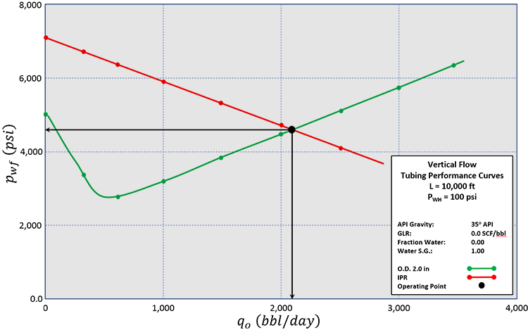
A hypothetical tubing performance curve for a 2.0 inch outer diameter (O.D. – remember, the I.D. of the tubing controls the pressure drop, but by convention we quote the tubing size by its outer diameter, O.D.) tubing is shown in Figure 7.21. In the legend of this figure, we see some of the static and dynamic properties that impact tubing performance (see Table 6.04). In particular, we can see the wellhead pressure, $p_{W H}$ , is 100 psi in this example/figure. This wellhead pressure would be the pressure on the gauge of the wellhead shown in Figure 7.13. The flowing well pressure, $p_{w f}$ , in this figure is the solution of the well hydraulics equations (Darcy-Weisbach Equation or multi-phase flow correlation) which represents the pressure at the bottom of the tubing string (y-axis on this plot) that is required to lift the reservoir fluids at a given production rate (x-axis on this plot).

Note, that we can rearrange Equation 7.01 and solve for $p_{w f}$ :

p_{w f} = p - \frac{q}{P I}

Equation 7.03

This is the equation for a straight line in $q$ with a slope of $- \frac{1}{P I}$ and a y-intercept of $p$ The pressure, $p$ , acting as the y-intercept is the average pressure in the reservoir (for pseudo-steady state flow) and would slowly drift downward as the reservoir pressure is depleted with production. For multi-phase flow, we would not get a straight line, but a curve. For our straight-line example, the IPR is the red line in Figure 7.21. The Inflow Performance Relationship (IPR) represents the rate that fluids can be supplied from the reservoir at a given flowing pressure, while the Tubing Performance Curve, TPC, represents the rate that fluids can be received by the tubing and lifted to the surface at a 100 psi $p_{W H}$ . The intersection of these two curves, then, represents the operating point for the well at this wellhead pressure.

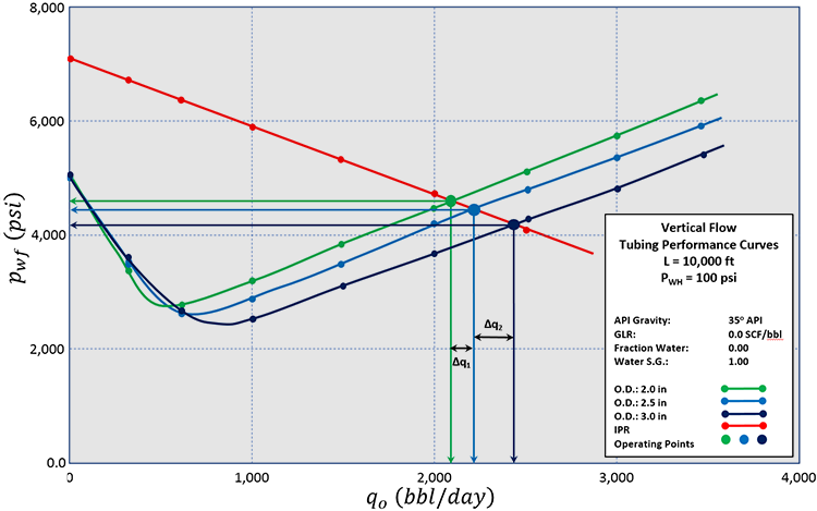
Figure 7.21: Inflow Performance Relationship (IPR), Tubing Performance Curve (TPC), and Operating Point for a Well

Source: Greg King © Penn State, licensed CC BY-NC-SA 4.0

If we were to build a well hydraulics model for a well to run sensitivities on the tubing size, then a plot such as Figure 7.22 would result. When I say “… build a well hydraulics model …”, this model can be a simple as a hand calculation model^[4] (the industry standard method thirty years ago), an Excel spreadsheet model, or a current generation software model. The details to include in such a model depend on the objectives of the model. Any well model built with an objective of aiding in the completion design would need to include any pressure losses associated with the completion (for example, pressure drop due to flow through the gravel pack, flow through the perforations, or flow through a hydraulic fracture). We will discuss some of these additional pressure drops later in this lesson.

For sizing the tubing of the well, we would simply be able to calculate the $Δ q's$ associated with going from one tubing size (O.D.) to the next incremental tubing size (O.D.), run the economics to determine if the larger, more expensive tubing size would pay for itself with its incremental production rate (meet corporate economic hurdles), and continue until we found a tubing size (O.D.) that was uneconomic or could not physically fit inside our production casing.

One example that we can use for estimation of the tubing size is the payback time for an incremental increase in the tubing size. The payback time is the time period required to recoup an investment (or, in other words, the time period that the investment ties up our money). If the incremental rate from the IPR-TPC analysis shown in Figure 7.22 is $Δ q_{o}$ (STB/day), the total incremental cost for increasing the tubing size is $Δ C_{T}$ ($), and oil price is $P_{o}$ ($/STB), then the payback time, $t_{P B}$ (days) is:

t_{P B} = \frac{Δ C_{T}}{P_{o} Δ q_{o}}

Equation 7.04

Figure 7.22: Inflow Performance Relationship and Tubing Size Sensitivities

In this equation, the numerator is the incremental cost of the larger tubing size in dollars, while the denominator represents the daily revenue of the incremental oil sales in $/day. If a detailed estimate of $t_{P B}$ is required, then we can allow the rate to change over time using the decline curve analysis methods discussed in Lesson 4 and Lesson 5 (rather than using a constant $Δ q_{o}$ based on stabilized rates).

Earlier, I used the phrase “… corporate economic hurdles …;” I can illustrate the concept of an economic hurdle with our definition of payback time, Equation 7.04. Perhaps the company that you work for dictates that all design aspects of the well must pay for themselves in one year or less; then, we could use the IPR-TPC analysis to determine the largest tubing size that yields a $t_{P B}$ from Equation 7.04 that meets this one-year threshold.

When sizing tubing, we must also be aware that there are other considerations to be evaluated. For example, if we plan to run logging tools on wireline or perform a through-tubing workover, then we would need to size the tubing so that the inner diameter, I.D., would be able to accommodate the physical dimensions of the tools that we plan to run plus any tolerances. From the tubing sizes used in this example, 2.0, 2.5, and 3.5 inch O.D., we can see that the dimensions used in oil and gas wells can be important design criteria for the tubing size selection.

[3] Rawlins, E.L. and Schellhardt, M.A. 1935. Backpressure Data on Natural Gas Wells and Their Application to Production Practices, 7. Monograph Series, U.S. Bureau of Mines.

[4] Brown, K.,E.: The Technology of Artificial Lift Methods (Vols. 1 – 4), Petroleum Publishing Co., Tulsa, O.K. (1977)

Navigation

EMS

Programs

Related Links