Lesson 6: Production Engineering: Flow in Well Tubing
6.0: Lesson Overview
You will have two weeks to complete Lesson 6.
Lesson 6 is very extensive, and you will have two weeks to read through the lesson and complete the associated assignments. Please use your time wisely and don't let yourself fall behind; you will need the extra week to work your way effectively through the material.
Please refer to the Calendar in Canvas for specific time frames and due dates.
In this lesson, we will discuss fluid flow in the oil and gas wells. Production Engineers are concerned with optimizing production from a given well. Well Modeling is a tool that allows production engineers to determine production rates and pressure drops in a well. This allows the engineer to identify bottlenecks in the production system (reservoir, tubing, well head) and seek methods to alleviate these bottlenecks (debottleneck the well).
Production engineers use tubing calculations and well modeling during all phases of the well’s productive life - from designing the initial completion to developing well intervention strategies as conditions in the reservoir change (pressure and saturations).
Learning Objectives
By the end of this lesson, you should be able to:
- list and understand the different well orientations used to produce crude oil and natural gas;
- describe the basics of tubing hydraulics (fluid flow in well tubing) during crude oil and natural gas production;
- state the physical parameters that impact pressure losses in well tubing;
- discuss the different flow regimes that can occur in vertical and horizontal flow through well tubing;
- explain the concept of the energy balance and how it relates to tubing hydraulics and the Darcy-Weisbach Equation;
- explain the concept of friction losses in well tubing and understand the factors that control frictional losses during production and injection;
- identify the equations that can be used to estimate the pressure drop in single-phase liquid and gas flow;
- perform tubing hydraulics calculations for single-phase liquid and gas flow;
- describe the differences between a Pressure Traverse Calculation and a Tubing Performance Calculation for single-phase and multi-phase flow;
- list and describe the static and dynamic data considered in tubing hydraulics calculations;
- describe the concept of a flow pattern map and how these maps are incorporated into multi-phase tubing hydraulics calculations; and
- list the different multi-phase flow correlations used in the oil and gas industry and their applications.
Lesson 6 Checklist
| To Read | Read the Lesson 6 online material | Click the Introduction link below to continue reading the Lesson 6 material |
|---|---|---|
| To Do | Lesson 6 Quiz | Take the Lesson 6 Quiz in Canvas |
Please refer to the Calendar in Canvas for specific time frames and due dates.
Questions?
If you have questions, please feel free to post them to the Course Q&A Discussion Board in Canvas. While you are there, feel free to post your own responses if you, too, are able to help a classmate.
6.1: Introduction
In earlier lessons, we learned that production engineers are tasked with optimizing the production or injection from individual wells. This optimization involves monitoring the well to determine if its performance can be improved; stimulating the well with acidizing or hydraulic fracturing if there is well damage; applying artificial lift (gas lift or pumps) to improve the economics of low rate wells; performing well workovers to shut-off excess gas or water production; along with many other types of well interventions.
In order to understand how wells are performing, we must first understand the tubing hydraulics (flow behavior in production or injection wells). For this, we need an introduction to modern oil and gas wells and a brief description of the nature of the problem to be solved.
6.2: Introduction to Gas and Liquid Flow through Well Tubing
In oil and gas production, Tubing is the pipe or conduit where fluids are transported from the reservoir to the surface. This is shown Figure 6.01. Figure 6.01 shows the Wellbore Schematic for a typical vertical well. This figure is a schematic cross-section through the axis of the well. This schematic shows two types of pipe, casing and tubing. The casing is used and installed during the drilling process, and we will discuss the purpose of the casing when we discuss the drilling process in Lesson 8. For now, we are interested in the tubing.
The tubing is the inner most string of pipe in the well. As I stated, this is the conduit that connects the reservoir to the surface. Reservoir fluids flow from the reservoir, through the perforations, into the tubing, and the up the well. In this well schematic, fluids are prevented from flowing through the Annular Space between the tubing and Production Casing String with a Packer (a packer is a device that seals the annular space between the production casing and tubing and mechanically prevents fluids from flowing through the annulus). It is the tubing that will be the focus of this lesson.

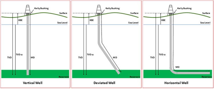
Wells drilled for oil and gas production (or fluid injection) are not always straight, vertical wells. Wells can be designed to be straight, deviated, or horizontal. This is shown in Figure 6.02 for three common well types: vertical wells, deviated wells, and horizontal wells. In addition to wells that were planned to be deviated, wells that were planned to be straight, vertical wells often deviate from the true vertical direction during the drilling process.
In the field, the measurement of the three-dimensional path of a well is called a Directional Survey. A directional survey can be performed with either magnetic or gyroscopic instrumentation. The data recorded during a directional survey include:
- the True Vertical Depth, TVD
- the Measured Depth, MD
- the well inclination from the vertical (0° for a vertical well and 90° for a horizontal well). Note, for our flow calculations, we will use inclination from the horizontal
- the well direction N-S-E-W or 0 - 360°)
The objectives of the directional survey are to:
- determine the exact bottom-hole location;
- monitor the well’s progress during drill to ensure the well will reach the intended target;
- orient the deflection of any tools run in the well to ensure tools can traverse the well path;
- establish the relationship of TVD and MD for in support of well logging and wellbore hydraulics modeling; and
- calculate the TVD of various geologic formations to allow for proper geological mapping.
Figure 6.02 depicts three wells. In this figure, the Kelly Bushing is the mechanical assembly that rotates on the rig floor causing the drill pipe and drill bit to rotate. We will learn much more about the Kelly Bushing in Lesson 8. The Kelly Bushing (and, essentially, the rig floor) is a common reference point for depths/lengths in a well. This figure shows four common measurements used in the oil and gas industry for the well lengths and depths:
- TVD: True Vertical Depth is the depth (or length) in the true vertical direction measured from the Kelly Bushing to the point of interest.
- TVD ss: True Vertical Depth sub-sea is the depth (or length) in the true vertical direction measured from the mean sea level to the point of interest.
- MD: Measured Depth is the path length of the depth (or length) measured from the Kelly Bushing to the point of interest.
- KBE: The Kelly Bushing Elevation is the elevation of the Kelly Bushing measured from the sea level.
As we will see, these measurements can have a significant impact on the tubing hydraulics once the well is put onto production or injection. For example, gravity (and hydrostatic pressure) and the geothermal gradient will act in the true vertical direction (TVD), while friction will act along the total length of the tubing (MD).
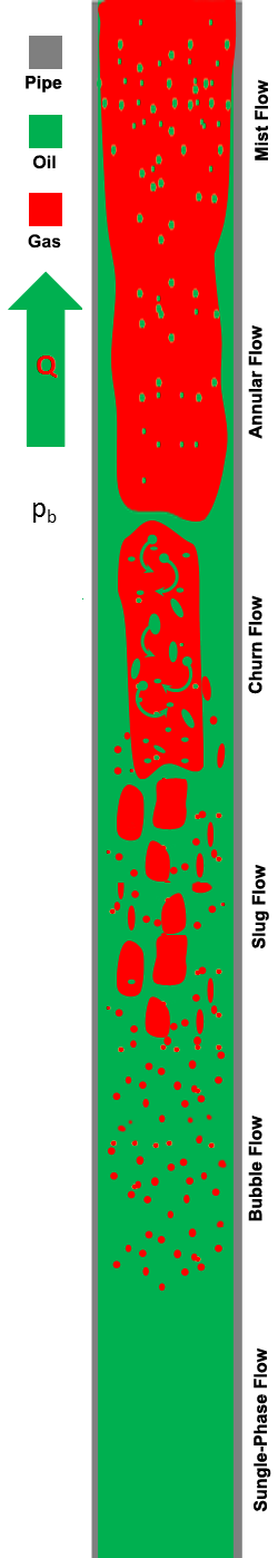
As oil enters the well and begin flow upwards several Flow Regimes or Flow Patterns can occur in the tubing. These flow patterns in vertical flow are shown in Table 6.01.
| Vertical Cross-section | Description |
|---|---|
 |
Mist Flow:
|
Annular Flow:
|
|
Churn Flow:
|
|
Slug Flow:
|
|
Bubble Flow:
|
|
Single-Phase Flow:
|
|
| Image by Greg King © Penn State, is licensed under CC BY-NC-SA 4.0 [1] | |
When crude oil first enters the well and tubing, it may be above its bubble-point pressure (note, if the reservoir is below the bubble-point pressure, then free gas will enter the well and tubing and a more continuous gas phase will be present in the base of the tubing near the perforations). As the liquid flows up the tubing, pressure is expended as a pressure differential is required to lift the liquid column to the surface.
At some point, the pressure falls below the bubble-point pressure in the tubing, and gas begins to come out of solution. As we discussed in Lesson 2, crude oils and natural gases are complex mixtures hydrocarbon molecules. Figure 6.03 is a Phase Diagram for an undersaturated oil reservoir (crude oil above its bubble-point pressure). In Lesson 4 and Lesson 5, we discussed the behavior of the crude oil and natural gas in the reservoir. This is the solid p-T path shown in Figure 6.03: Path (, ) to (, ).
The dashed p-T path in Figure 6.03 is the path that the fluids take going from the reservoir to the surface separator. Remember, we have seen in Lesson 4 and Lesson 5 that in the reservoir as we remove fluids, the reservoir pressure is reduced. Therefore, the starting point for the path to the separators, Path (, ) to (, , will be the time-dependent current reservoir pressure,
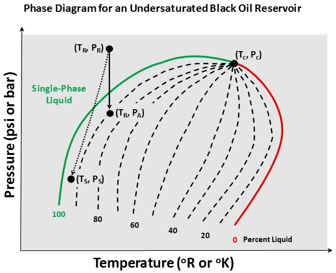
As fluids travel up the well along the dashed path in Figure 6.03, we can see that the tubing flow is a non-isothermal process; the temperature of the flowing fluid changes due to the local geothermal gradient. This has several implications in the tubing hydraulics process. For example, as we see in Figure 6.03, the bubble-point pressure (the pressure where the path enters the two-phase region) for the solid reservoir path, Path (, ) to (, ), is different from the bubble-point pressure for the dashed tubing path, Path (, ) to (, ). It is the bubble-point pressure along the dashed path that results in the onset of the bubble flow pattern shown in Table 6.01.
As flow continues up the tubing in Table 6.01, the pressure continues to fall causing gas bubbles to expand due to the compressible nature of gas and solution gas to come out of solution. As the gas bubbles expand, they begin to coalesce and form gas slugs in the center of the tubing. Due to buoyancy, the gas slugs travel at a higher velocity than the liquid and begin to push the liquid up the tubing.
As flow continues up the tubing, the gas slugs continue to expand and begin to form a continuous phase in the center of the tubing. This is the churn flow pattern shown in Table 6.01. During churn flow, high velocity gas pushes liquids up the well, but liquid tends to slip back downward due to its density. As flow continues upward, the continuous gas phase pushes the liquid up the tubing with gas flowing rapidly in the center of the tubing and the liquid flowing slower in the annular space between the tubing walls and the continuous gas phase. This is the annular flow pattern shown in Table 6.01.
As gas and liquid continue to flow upward, the gas phase expands further, leaving less room on the tubing walls for the liquid. During this flow regime, liquids are pushed upwards in liquid slugs and as mist entrained in the gas.
We should remember that not all of these flow regimes occur in all wells. The flow regimes occurring in the tubing will be determined by the conditions in the well. For example, if an undersaturated crude oil reservoir is being produced and the wellhead pressure, , is kept above the surface bubble-point pressure, then the well will only flow in the single-phase flow regime.
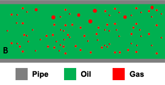
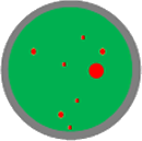
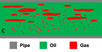
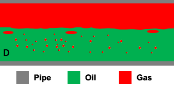
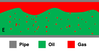
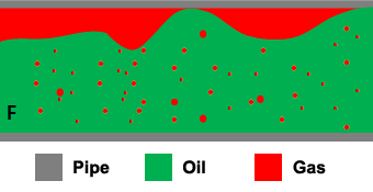
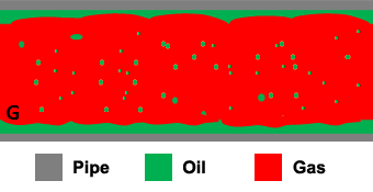
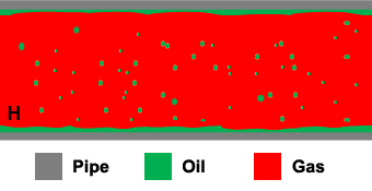
As we can see from Figure 6.02, wells can be planned and executed as deviated (or slanted) wells and as horizontal wells. Flow through the tubing in the horizontal section of a well has distinct flow patterns. These flow patterns are illustrated in Table 6.02.
| Cross-Section | Longitudinal-Section | Description |
|---|---|---|
 |
 |
Single-Phase Flow:
|
 |
 |
Bubble Flow:
|
 |
 |
Plug Flow:
|
 |
 |
Stratified Flow:
|
 |
 |
Wavy Flow:
|
 |
 |
Slug Flow:
|
 |
 |
Annular Flow:
|
 |
 |
Spray Flow:
|
|
Source: All images by Greg King © Penn State, licensed under CC BY-NC-SA 4.0 [1]
|
||
Referring to Table 6.02, as with vertical tubing, if oil enters the horizontal tubing above the bubble-point pressure, then flow will be single-phase and the liquid will be transported in the Single-Phase Flow Regime. As pressure travels horizontally, the pressure differential required to transport the liquid may cause the pressure to drop below the bubble-point pressure of the oil. When this occurs, the tubing fluids enter the Bubble Flow Regime (B). As pressure drops further due to liquid transport, the bubbles expand and coalesce to form gas plugs. When this occurs, the gas and liquid enter the Plug Flow Regime (C). As pressures continue to drop, the gas plugs continue to expand and coalesce, eventually forming a continuous gas phase. If the phase velocities are low, then gravity will act to segregate the phases vertically. This is the Segregated Flow Regime (D). In the segregated flow regime, the surface between the two phases is relatively smooth. If velocities are higher, then the surface of the two segregated phases may develop waves and ripples. This is the Wavy Flow Regime (E). If the velocities are greater still, then the height of the waves may reach the top of the tubing, temporarily closing off the cross-section to the flow of gas. This is the Slug Flow Regime (F). The slug flow regime results in very unstable flow because of the differences in the momentum between the gas and liquid phases due to the different densities and different phase velocities. When the cross-section is cut off to the gas phase, its momentum must be transferred to the liquid phase. At higher velocities, gravity acts too slow to segregate the phases and the flow may enter the Annular Flow Regime (G). In this flow regime, the continuous gas phase occupies the center of the tubing, while liquid phase forms an annular ring between the gas phase and the tubing wall. While gravity may be too slow to create complete vertical segregation, the less dense gas phase may flow higher in the tubing (i.e., the gas and oil may flow in a non-concentric manner). Finally, if the velocity is very high, the gas may occupy most of the cross-section and liquid is transported as a mist that is entrained in the gas. This occurs in the Spray Flow Regime (H). Spray flow is a very stable flow regime with the liquid and gas phases traveling at comparable velocities.
These are the basic flow regimes that can occur in vertical and horizontal tubing. We will revisit these flow regimes when we discuss Multi-Phase Tubing Performance later in this lesson.
6.3: Tubing/Pipe Calculations
6.3: Tubing/Pipe Calculations section of this lesson will cover the following topics and sub-topics:
- 6.3.1: Equations Governing Flow in Pipe and Tubing [2]
- 6.3.2: Single-Phase Flow of Liquids in Tubing [3]
- 6.3.2.1: The Darcy-Weisbach Equation for Single-Segment Oil Production Wells [4]
- 6.3.2.2: The Darcy-Weisbach Equation for Segmented Oil Production Wells [5]
- 6.3.2.3: The Darcy-Weisbach Equation for Segmented Injection Wells [6]
- 6.3.2.4: The Hazen-Williams Equation for Liquid Production/Injection Wells [7]
- 6.3.3: Single-Phase Flow of Gases in Tubing [8]
- 6.3.4: Multi-Phase Flow [11]
6.3.1: Equations Governing Flow in Pipe and Tubing
Bernoulli’s Equation
Bernoulli’s Equation forms the basis of the steady-state tubing performance. Bernoulli’s Equation is simply an energy balance on a given system. In our case, that system is the production tubing. Bernoulli’s Equation can be written as:
In this equation, all of the terms have the units of lbf-ft. The variables in this equation are:
- and are the Internal Energies stored in the fluid at two points in the system, lbf-ft. This internal energy is energy at the molecular level and cannot be measured in an absolute sense. We can establish the relative change in the internal energy () by assigning a zero value at some specific set conditions.
- and are the pressures at two points in the system, psi
- and are the volumes of the fluid at two points in the system, ft3
- The terms and are the Energies of Expansion or Compression, lbf-ft. These terms represent compressional energy stored in the fluid (similar to the energy stored in a compressed spring).
- is the mass of the fluid in the system, lbm
- and are the velocities of the fluid at two points in the system, ft/sec
- is the Universal Gravitational Constant, 32.174 lbm-ft/lbf-sec2
- The terms and are the Kinetic Energy of the fluid in the system, lbf-ft
- is the Local Acceleration due to gravity, ft/sec2. The local acceleration due to gravity varies from location to location but is approximately equal to 32.174 ft/sec2. The ratio of is approximately equal to 1.0 lbf/lbm.
- and are elevations above some reference point, typically sea level, ft
- The terms and are the Potential Energies of the fluid at two points in the system, lbf-ft
- is the Thermal Energy added to or removed from the system, lbf-ft. In Equation 6.01, is positive if thermal energy is added to the system or negative if thermal energy is removed from the system (note: 1 BTU = 778.169 lbf-ft)
- is the work added to or performed by the fluid, lbf-ft. In Equation 6.01, is positive if work is added to the system (for example, with a pump) or negative if work is removed from the system (for example, by turning a turbine)
There are many engineering Thermodynamics concepts in this equation which are out-of-scope for this course; however, we can illustrate the application of Bernoulli’s Equation in the context of flow through tubing with Figure 6.04.
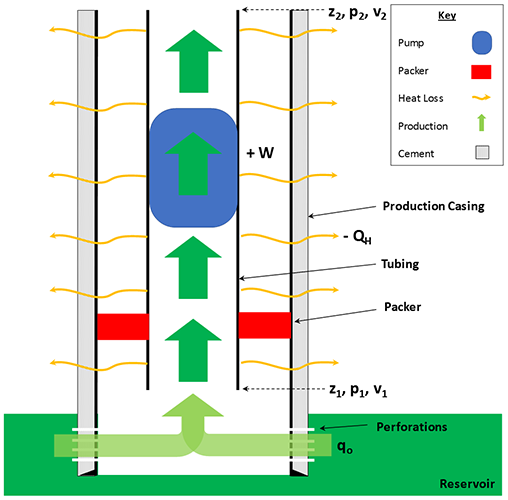
In Figure 6.04, we have a length of vertical tubing defined from a depth of to a depth of with an inner diameter of . A mass of oil enters the tubing at at a volumetric rate of (ft3/sec) at a pressure of and a velocity of . As the oil travels up from the reservoir, the surrounding rock is cooler than the oil due to the local geothermal gradient, and heat is lost () from the hot oil to the surrounding cooler rock. Flowing upward, the oil encounters a downhole pump which supplies work () to the system. The oil finally reaches point in the tubing with a Terminal Pressure of and Terminal Velocity of .
Without going into the thermodynamic details, Equation 6.01 can be rewritten in differential form as:
Where:
and,
- is the pressure at a point in the tubing, psi
- is the distance along the axis of the tubing, ft
- 144 is a unit conversion constant, in2/ft2
- 12 is a unit conversion constant, in/ft
- is the Universal Gravitational Constant, 32.174 lbm-ft/lbf-sec2
- is the Local Acceleration due to gravity, ft/sec2. The local acceleration due to gravity varies from location to location but is approximately 32.174 ft/sec2. The ratio of is approximately 1.0 lbf/lbm
- is the angle of inclination above the horizontal, dimensionless
- is the Darcy-Weisbach Friction Factor, dimensionless
- is the velocity of the fluid at the point in the tubing, ft/sec
- is the density of the fluid, lbm/ft3
- is the Inner Diameter () of the tubing, in
- is the elevation of the point in the tubing above a reference point, typically sea level, ft
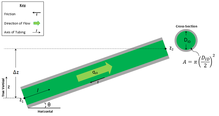
The units of each of the terms in Equation 6.02 and Equation 6.03 are psi/ft. The well orientation for Equation 6.02 and Equation 6.03 is shown in Figure 6.05.
In Equation 6.02, I have neglected the Heat Transfer, , and Work, , terms. If we have significant heat transfer or a device that adds or performs work, we can include these terms into the equation.
Expanding on the terms in Equation 6.02, the elevation term, , is simply the change in the potential energy as the fluid flows through the tubing in the direction of . Note that in the convention shown in Figure 6.05 with the z-direction upward, point has a higher potential energy than point because it has a higher elevation. The friction term, , is the irreversible loss of energy due to friction as the fluid flows past the stationary tubing wall. Friction always acts in the direction of opposite of flow. For single-phase flow, the only friction component occurs at the liquid-tubing interface. In multi-phase flow where phases are flowing at different velocities, there will be a friction component occurring at the phase boundaries also. Finally, the acceleration term, , is the change in energy resulting from the acceleration or deceleration of the fluid going around bends in the tubing. The acceleration term is often neglected in tubing calculations.
As mentioned earlier, the friction factor, fDW, in Equation 6.03b is the Darcy-Weisbach friction factor. This equation is co-credited to Henry Darcy, who is the same Darcy that gave us Darcy’s Law. The Darcy-Weisbach friction factor is the ratio of the shear stress at the wall and the kinetic energy of the fluid on a unit volume basis. This friction factor was plotted by Moody[1]as a function of the Reynolds Number[2],[3], , and the Relative Roughness . The Moody Diagram is shown in Figure 6.06.
Note, we will be using the Darcy-Weisbach friction factor, , which is not to be confused with the Fanning Friction Factor, [4]. The Fanning friction factor is ¼ the value of the Darcy-Weisbach friction factor, that is: . The difference between the two friction factors is that the Darcy-Weisbach friction factor is typically used for closed circular pipes, and uses as the diameter, while the Fanning friction factor can be used for open conduits and uses the concept of the “hydraulic radius” as a measure of the diameter: . Where is the hydraulic radius, is the cross-sectional area of flow (length squared), and is the “wetted perimeter” (length). The wetted perimeter is the perimeter of the cross-section in contact with the conduit (portion of the cross-section that is “wetted” by the fluid).
The Reynolds Number, , is a dimensionless group that represents the ratio of the inertial forces to the viscous forces within the fluid and is used to characterize laminar and turbulent flow regimes. For our application of flow through pipe, the Reynolds Number is defined by:
Where:
- is the Reynolds Number, dimensionless
- 1488.0 is a unit conversion constant, ft-sec-cp/lbm
- 12 is a unit conversion constant, in/ft
- 124 in an equation constant
- is the Inner Diameter ( ) of the tubing, in
- is the velocity of the fluid in the tubing, ft/sec
- is the density of the fluid, lbm/ft3
- is the dynamic viscosity of the fluid, cp
Note, Equation 6.04a can be expressed in an equivalent form in terms of flow rate, :
Where the velocity term was replaced with the rate term: .
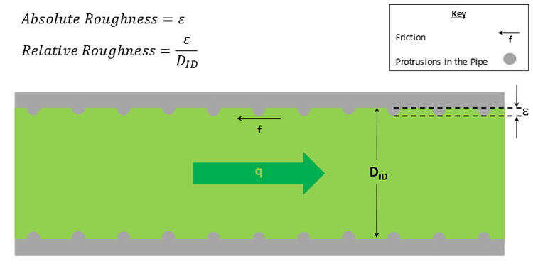
At lower values of flow is in the laminar flow regime, while at higher values of flow is in the turbulent flow regime. As we see in the Moody Diagram, Figure 6.06, in the turbulent flow regime the friction factor is a function of the Reynolds Number and relative roughness of the pipe . The relative roughness is a dimensionless quantity that is defined as the length of protrusions (lumps, pipe defects and imperfections, pits from corrosion, etc.) divided by the inner diameter of the tubing. It is a measure of the departure of an actual steel pipe from an idealized, smooth pipe. Figure 6.07 illustrates the concepts of absolute and relative roughness, while Table 6.03 shows typical values of the absolute roughness, , for different materials.
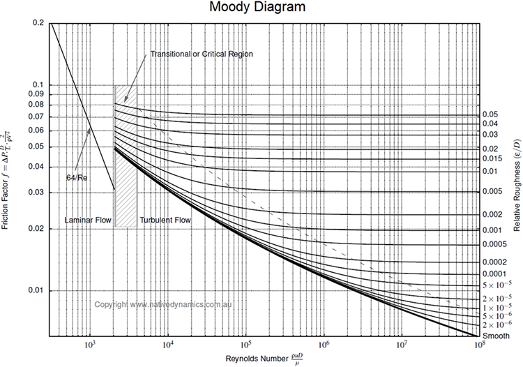
In the laminar flow regime , the Darcy-Weisbach friction factor is a function of the Reynolds Number only and can be determined by:
| Material | ||
|---|---|---|
| Idealized smooth surface – any material | 0.0 | 0.0 |
| Concrete – coarse | 0.2500 | 0.009842 |
| Concrete – new smooth | 0.0250 | 0.000984 |
| Drawn tubing | 0.0025 | 0.000098 |
| Glass, Plastic Perspex | 0.0025 | 0.000098 |
| Iron – cast | 0.1500 | 0.005906 |
| Sewers – old | 3.0000 | 0.118110 |
| Steel – mortar lined | 0.1000 | 0.003937 |
| Steel – rusted | 0.5000 | 0.019685 |
| Steel – structural or forged | 0.2500 | 0.009842 |
| Water mains – old | 1.0000 | 0.039370 |
As previously discussed, in the turbulent flow regime, the Darcy-Weisbach friction factor is a function of both the Reynolds Number and the relative roughness. To calculate the friction factor in the turbulent regime, the Implicit Colebrook Equation[6] can be used:
We say that this equation is implicit because the friction factor, , appears on both sides of the equals sign. Therefore, to solve this equation, we must iterate on a solution. That is, we make an initial guess at and use it on the right-hand side of the equation to calculate a new on the left-hand side of the equation. We repeat this process until the two values of (the recently calculated value on the left-hand side of the equation and the value used in the calculation on the right-hand side of the equation) are sufficiently close. To start the process, an Explicit Formula for , such as the Swamee-Jain Equation[7], is used:
We say that Equation 6.07 is an explicit formula because the friction factor does nor appear on the right-hand side of the equation, and we can solve for it explicitly. The Swamee-Jain Equation[7] is an approximation to the Colebrook Equation[6] and can also be used directly in calculations.
[1] Moody, L. F. (1944), "Friction factors for pipe flow", Transactions of the ASME, 66 (8): 671–684
[2] Stokes, George (1851). "On the Effect of the Internal Friction of Fluids on the Motion of Pendulums". Transactions of the Cambridge Philosophical Society. 9: 8–106.
[3] Reynolds, Osborne (1883). "An experimental investigation of the circumstances which determine whether the motion of water shall be direct or sinuous, and of the law of resistance in parallel channels". Philosophical Transactions of the Royal Society. 174 (0): 935–982.
[4] Fanning, J. T. (1877). A practical treatise on water-supply engineering, Van Nostrand, New York, 619
[6] Colebrook, C. F. (1938–1939). "Turbulent Flow in Pipes, With Particular Reference to the Transition Region Between the Smooth and Rough Pipe Laws". Journal of the Institution of Civil Engineers. London, England. 11: 133–156.
[7] Swamee, P.K., and Jain, A.K. (1976). Explicit equations for pipe flow problems. J. Hydraul. Div. ASCE 102 (HY5), 657–664.
6.3.2: Single-Phase Flow of Liquids in Tubing
6.3.2: Single-Phase Flow of Liquids in Tubing section of this lesson will cover the following topics:
- 6.3.2.1: The Darcy-Weisbach Equation for Single-Segment Oil Production Wells [4]
- 6.3.2.2: The Darcy-Weisbach Equation for Segmented Oil Production Wells [5]
- 6.3.2.3: The Darcy-Weisbach Equation for Segmented Injection Wells [6]
- 6.3.2.4: The Hazen-Williams Equation for Liquid Production/Injection Wells [7]
6.3.2.1: The Darcy-Weisbach Equation for Single-Segment Oil Production Wells
The Darcy-Weisbach Equation is one of the most common equations for modeling single-phase liquid flow through pipes and tubing. The Darcy-Weisbach Equation is developed by ignoring the acceleration term in Equation 6.02 and replacing the derivative with a finite-difference approximation:
Where the angle, , is measured from the horizontal and is 90º for true vertical wells and 0º for horizontal wells. Solving this equation for the velocity:
Substituting for the velocity term, :
or, after evaluating the constants and rearranging:
Noting that the term (the change in elevation over the length of the tubing, ):
This is the theoretically derived Darcy-Weisbach Equation for flow through pipe/tubing in oilfield units. This equation relates the flow rate, , to a given pressure drop . In practice, we include a dimensionless efficiency factor, , which is approximately equal to one . This efficiency factor is used to tune the equation to actual field measurements.
This version of the Darcy-Weisbach Equation is the version most often used in industry software. In this equation:
- 411.147 is an equation constant
- 144 is a unit conversion constant, in2/ft2
- is the flow rate through the tubing, bbl/day
- is an efficiency (tuning) factor for the tubing section , dimensionless
- is the Inner Diameter () of the tubing, in
- is the Universal Gravitational Constant, 32.174 lbm-ft/lbf-sec2
- is the Local Acceleration due to gravity, ft/sec2. The local acceleration due to gravity varies from location to location but is approximately 32.174 ft/sec2. The ratio of is approximately 1.0 lbf/lbm
- is the Darcy-Weisbach Friction Factor, dimensionless
- is the density of the fluid, lbm/ft3
- is the length of the section of tubing along its axis, ft
- and are the pressures at two points in a section of tubing, psi
- and are the elevations at two points in a section of tubing, psi
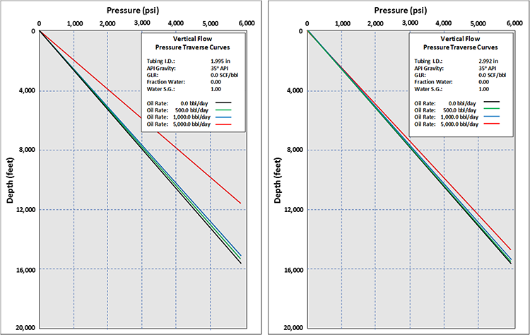
We can use this equation in two ways. The first way to use Equation 6.12, is to specify the flow rate and calculate the pressure drop along the section of the pipe/tubing. This calculation is called a Pressure Traverse calculation and is illustrated in Figure 6.08 for a vertical well. In this figure, two tubing diameters are considered, and multiple production rates are plotted for each tubing size. The pressure traverse calculation is used by production engineers to help select the appropriate tubing size for the anticipated well production rates during the completion design phase of the well.
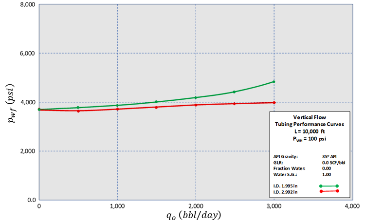
Alternatively, if we know one pressure and the flow rate, then we can calculate the other pressure. This is normally done by specifying the Well Head Pressure, , and calculating the flowing bottom-hole pressure, , for multiple production rates. This is called Tubing Performance calculation and is illustrated in Figure 6.09 for a well head pressure of and the same two tubing sizes plotted in Figure 6.08: in and .
6.3.2.2: The Darcy-Weisbach Equation for Segmented Oil Production Wells
In our previous discussion, we assumed that properties, such as, viscosity and density (for use in the Reynolds Number calculation in Equation 6.04) or the density (for use in the Darcy-Weisbach Equation itself in Equation 6.12) were constant over the entire length of the pipe/tubing. As fluids flow up the vertical section of tubing, the pressure drop may cause changes in these properties for slightly compressible fluids. In addition, the upward flow of fluids in the vertical section of tubing is a non-isothermal process, and this may also cause changes in these properties as fluids flow upward. As already mentioned, in the extreme case, fluids may drop below the bubble-point pressure, resulting in multi-phase flow through multiple flow regimes (see Table 6.01). For these cases, Segmented Wells can be used.
Segmented wells are wells where the entire well length is partitioned into multiple, smaller well segments. The pressure drop along one segment is calculated using the local pressure and temperature conditions (assuming an appropriate heat transfer model is available). Once the calculations are performed for one segment of tubing, the Terminal Pressure (pressure at the outlet end of the tubing section - in Figure 6.04) is used as the starting pressure (or inlet pressure, ) for the next segment of the well.
In addition to fluid property changes during flow, there may be design reasons for using segmented wells. For example, the deviated and horizontal wells shown in Figure 6.02 will require the use of segmented wells: at least one segment for the non-vertical section of the tubing and at least one segment for the vertical section of the tubing. In addition, there may be reasons for designing a Tapered Tubing String (a tubing string with different inner diameter tubing sizes along different lengths of the well). These wells are designed to keep a desired flow velocity at different depths in the well.
The use of segmented wells for modeling well production is the most common method of modeling actual wells. Well modeling is a common activity for Production Engineers.
6.3.2.3: The Darcy-Weisbach Equation for Segmented Injection Wells
Injection Wells are required for Secondary and Tertiary Oil Production Methods. In secondary and tertiary production, fluids are pumped from the surface and injected into the reservoir. The most common secondary oil production method is Waterflooding. For the purpose of our discussion, this is relevant because the direction of the fluid is reversed in Figure 6.04 and Figure 6.05, resulting in a reversal of the signs in our equations. Therefore, for liquid injection wells, the Darcy-Weisbach Equation becomes (note sign change):
6.3.2.4: The Hazen-Williams Equation for Liquid Production/Injection Wells
In addition to the Darcy-Weisbach Equation for liquid production/injection wells, the Hazen-Williams Equation also has applications in the oil and gas industry (most commonly for injection wells, but also valid for light hydrocarbon liquids). The Hazen-Williams Equation is an Empirical Method (based on observations, not theory) which pre-dates the Darcy-Weisbach Equation. It was used in times prior to the widespread use of computers due to its simplicity, as it does not include a friction factor. The Hazen-Williams formula replaces the general friction factor with a material specific constant, , and modifies the equation constant and exponents. The Hazen-Williams Equation in oilfield units is:
In this equation:
- 15.2 is an equation constant
- 144 is a unit conversion constant, in2/ft2
- is the sign convention used in the equation with “ ” for production or “ ” for injection
- is the flow rate through the tubing, bbl/day
- is the Hazen-Williams (tuning) Factor for the tubing section , dimensionless
- is the Inner Diameter ( ) of the tubing, in
- is the Universal Gravitational Constant, 32.174 lbm-ft/lbf-sec2
- is the Local Acceleration due to gravity, ft/sec2. The local acceleration due to gravity varies from location to location but is approximately 32.174 ft/sec2. The ratio of is approximately 1.0 lbf/lbm
- is the density of the fluid, lbm/ft3
- is the length of the section of tubing along its axis, ft
- and are the pressures at two points in a section of tubing, psi
- and are the elevations at two points in a section of tubing, psi
Note in the Hazen-Williams Equation, that we have replaced the efficiency factor, , with the Hazen-Williams Factor, , and removed the friction factor, (in addition to modifying the constant and exponents). Typical values of for different materials are listed in Table 6.04. While the Hazen-Williams Factor is not an efficiency factor; in practice, it is used in much the same way as in the Darcy-Weisbach Equation: to tune the equation to match field measured data.
The computational simplicity of the Hazen-Williams Equation now becomes apparent – there is no need for the Reynolds Number and friction factor calculations. These calculations are included implicitly in the empirical Hazen-Williams Factor and the modified exponents. As mentioned earlier, the Hazen-Williams Equation is valid for water and light hydrocarbons, such as, gasoline and possibly condensates.
| Material | Minimum Value | Maximum Value |
|---|---|---|
| Polyvinyl chloride (PVC) | 150 | 150 |
| Fiber reinforced plastic (FRP) | 150 | 150 |
| Polyethylene | 140 | 140 |
| Cement, Mortar Lined Ductile Iron Pipe | 140 | 140 |
| Asbestos, cement | 140 | 140 |
| Copper | 130 | 140 |
| Cast iron – new | 130 | 130 |
| Galvanized iron | 120 | 120 |
| Cast iron – 10 years | 107 | 113 |
| Concrete | 100 | 140 |
| Steel | 90 | 110 |
| Cast iron – 20 years | 89 | 100 |
| Cast iron – 30 years | 75 | 90 |
| Cast iron – 40 years | 64 | 83 |
[8] Wikipedia: Hazen–Williams Equation [14]
6.3.3: Single-Phase Flow of Gases in Tubing
6.3.3: Single-Phase Flow of Gases in Tubing section of this lesson will cover the following topics:
6.3.3.1: The Darcy-Weisbach Equation for Gas Production Wells
The Darcy-Weisbach Equation for natural gases can be developed by modifying the equation for liquids using a simple change of units. For standard oilfield units:
or,
Note, this equation assumes that the flow rate, , is in ft3/day; however, it can easily be re-written in M ft3/day or MM ft3/day by adjusting the equation constant, 2,308.59, to either 2.30859 or 2.30859x10⁻³, respectively. In this equation:
- 411.147 is an equation constant
- 5.615 is a unit conversion constant, ft3/bbl
- Equation constant:
- 2,308.59 (for ft3/day)
- 2.30859 (for M ft3/day)
- 2.30859 x10⁻³ (for MM ft3/day)
- 144 is a unit conversion constant, in2/ft2
- is the sign convention used in the equation with “ ” for production or “ ” for injection
- is the flow rate through the tubing, ft3/day, M ft3/day, or MM ft3/day
- is an efficiency (tuning) factor for the tubing section, dimensionless
- is the Inner Diameter ( ) of the tubing, in
- is the Universal Gravitational Constant, 32.174 lbm-ft/lbf-sec2
- is the Local Acceleration due to gravity, ft/sec2.
- is the Darcy-Weisbach Friction Factor, dimensionless
- is the density of the fluid, lbm/ft3
- is the length of the section of tubing along its axis, ft
- and are the pressures at two points in a section of tubing, psi
- and are the elevations at two points in a section of tubing, psi
In Lesson 3, we saw that the density of a real gas could be determined by the Real Gas Law (Equation 3.71):
Due to the strong dependence of the gas density on local pressure and temperature, the solution of Equation 6.15b is always performed using the segmented well approach with iterations on the outlet pressure, . Essentially, the segmented well approach explicitly performs a numerical integration of the differential energy balance equation, Equation 6.08 (in terms of ). The steps for this simple iteration are:
- Assume a fixed length, , of tubing (usually in the range of 100 – 200 ft)
- Calculate the temperature (in ºR) halfway up the tubing length using the local temperature gradient in ºR/ft (feet in true vertical depth, )
- Start with the known inlet pressure,
- Assume an outlet pressure,
- Calculate the average pressure in the length of tubing,
- Calculate the Z-Factor and gas density from Equation 6.16 with the temperature from Step 2 and the average pressure from Step 5
- Evaluate the Reynolds Number from Equation 6.04 using this gas density (viscosity may also change with temperature)
- Calculate the Darcy-Weisbach Friction Factor from the Moody Diagram (Figure 6.06), the Colebrook Formula[6] (Equation 6.06), or the Swamee-Jain Equation[7] (Equation 6.07) using the Reynolds Number from Step 7
- Apply the Darcy-Weisbach Equation, Equation 6.15b, to calculate a new outlet pressure,
- Go to Step 5 and continue calculations until two successive iterations of agree to a specified tolerance
- When converged, proceed to the next length of tubing and start from Step 10
6.3.3.2: Other Equations for Gas Production Wells
As seen with this iteration, the use of the Darcy-Weisbach Equation can result in very complicated iteration process and requires the use of a computer for a solution. There are other methods available for gas wells and pipelines that can also be used that do not require an iteration.
One popular method used for gas wells is the Cullender and Smith[9] Method. This method uses a limited range of the relative roughness of 0.0006 to 0.00065 and a specialized friction factor correlation designed specifically for this range (not the generalized Colebrook Formula[6] or the Swamee-Jain Equation[7]). In addition, the method uses a two-step integration based on the trapezoid rule (two well segments). This method also requires an iteration, but it is not as complex as that shown above.
Other popular methods for gas wells and transmission lines include the Weymouth equation, the Panhandle “A” equation, and the Panhandle “B” equation. These equations are empirical equations developed from the generalized energy balance equation but use specialized, explicit friction factor correlations which allow them to be solved in a non-iterative manner. Also note that these equations use the flow rate in SCF/day and not ft3/day as in Equation 6.15. These equations have the form:
with
Where:
- is an equation constant:
- 433.5 (for the Weymouth equation)
- 435.87 (for the Panhandle “A” equation)
- 737.0 (for the Panhandle “B” equation)
- 0.0375 is an equation constant
- 5280.0 is a unit conversion constant, ft/mile
- is the flow rate through the tubing, SCF/day
- is an efficiency (tuning) factor for the tubing section , dimensionless
- is the Inner Diameter of the tubing, in
- is the standard temperature, ºR
- is the standard pressure, psi
- and are the pressures at two points in a section of tubing, psi
- is the specific gravity of the gas, , dimensionless
- is the real gas supercompressibility factor (Z-Factor), dimensionless
- is the average temperature of the tubing section, ºR
- is the length of the section of tubing along its axis, ft
- is a correction factor for change in elevation, dimensionless
- and are the elevations at two points in a section of tubing, ft
- is the angle from the horizontal, degrees or radians
- is an exponent:
- 2.667 (for the Weymouth equation)
- 2.6182 (for the Panhandle “A” equation)
- 2.530 (for the Panhandle “B” equation)
- is an exponent:
- 1.0 (for the Weymouth equation)
- 1.0788 (for the Panhandle “A” equation)
- 1.02 (for the Panhandle “B” equation)
- is an exponent:
- 1.0 (for the Weymouth equation)
- 0.853 (for the Panhandle “A” equation)
- 0.961 (for the Panhandle “B” equation)
- is an exponent:
- 0.5 (for the Weymouth equation)
- 0.5392 (for the Panhandle “A” equation)
- 0.51 (for the Panhandle “B” equation)
In these equations, the Z-Factor can is evaluated at the average pressure, :
Some investigators suggest that a more representative definition of average pressure, and hence a more accurate result, can be obtained with the following definition of average pressure:
When both the inlet pressure and the outlet pressure are known and the rate is the unknown, these equations (the Weymouth equation, the Panhandle “A” equation, and the Panhandle “B” equation) do not need an iteration for a solution. However, if the rate and one pressure are known and the other pressure is the unknown, then an iteration is still required. These equations can be used for tubing calculations or for calculations on long gas transmission pipelines. You will most likely see options for them if you use industry pipe flow or Nodal Analysis software. (Nodal Analysis is a well optimization technique where all components, or nodes, of the production system are modeled – the reservoir, skin, tubing, wellhead choke, flow line, and surface facilities – to identify any bottlenecks in the system for possible remediation or Debottlenecking.) For well modeling applications, Equation 6.17 through Equation 6.19 can be used to evaluate the pressure loss in the wells, in the Flow Lines (small ID pipe used to transport produced oil or gas from the wellhead to a gathering station, field separator, or other surface facility), and in gas transmission lines.
[9] Cullender, M.H., Smith, R.Y.: ''Practical Solution of Gas-Flow Equations for Wells and Pipelines with Large Temperature Gradients," Trans., AIME, 1956, vol. 207, p. 281.
6.3.4: Multi-Phase Flow
Well Modeling
Well Modeling is the process of developing models (supplying input) for actual wells and using these data in Well Modeling Software to perform the analyses required by the engineer. In all of our discussions to this point, we have assumed single-phase flow of either liquid or gas. Pressure loss calculations in multi-phase flow are much more complicated than those for single-phase flow. This is because in single-phase flow, the only frictional losses that occur in the system are at the fluid-pipe interface. In multi-phase flow, there is also the friction loss between the phases. As we have also seen in our discussion on flow regimes in tubing, there are multiple flow regimes that can occur in vertical, deviated, and horizontal wells and these can have a significant impact of energy and momentum transfer.
To quantify the pressure losses occurring in multi-phase flow calculations, we must consider the physics that are occurring in each flow regime. Typically, in the oil and gas industry, for multi-phase flow we evaluate the physics empirically. Table 6.05 lists the important physical data that have been observed to have a significant impact on the pressure drop in well tubing. These empirical physics are input into the well model with a Multi-Phase Flow Correlation.
There are many multi-phase flow correlations available and most pipe flow or nodal analysis software contains options for the most relevant correlations for crude oil and natural gas flow. The details of these multi-phase flow correlations are beyond the scope of this class, so I will briefly give a general description of them and then discuss the common correlations used in the oil and gas industry.
Well Model Data
As we have already discussed, the energy balance is a steady-state equation while our flow calculations are unsteady-state problems. When we use the energy balance equation to solve unsteady-state problems, we are solving a category of physical problems called a Series of Steady-States where the equation is derived for steady-state conditions, but we are solving it with time-dependent input data.
In Table 6.05 there are color coded entries: some of the data I have listed as Static Data which implies they do not change with time or location. Other data I have listed as Dynamic Data which implies that they may change with time, location, or both.
The entries in the green cells (Table 6.05 rows 1-6) are the data that make up a Well Model. These data are entered into the well modeling software and are treated as fixed data for some time period or some length of tubing. For example, I have already mentioned tapered tubing strings where the diameter of the tubing may change with position. When a well model is constructed, these design changes can be implemented as part of the segmented well model.
| Data or Property | Symbol | Description |
|---|---|---|
| Tubing/Pipe Diameter | Dynamic data but treated as static data | |
| Downhole well equipment | Pumps, chokes, etc. | Static data |
| True vertical depth, TVD | Vertical depth – depth in the true vertical direction | |
| Measured depth, MD | Measured depth – physical length of tubing | |
| Absolute or Relative Roughness | Dynamic data but treated as static data | |
| Efficiency | Dynamic data but treated as static data | |
| Liquid Hold-Up | Dynamic data: fraction of a representative elemental volume (REV) occupied by liquid (analogous to liquid saturation in the reservoir). | |
| Gas Hold-Up | Dynamic data: fraction of a representative elemental volume (REV) occupied by gas (analogous to gas saturation in the reservoir). | |
| Slip (or Slip Velocity) | Dynamic data (difference between velocities of two different phases). | |
| Gas-Liquid Ratio | Dynamic data: used as input to our pressure traverse or tubing performance calculation. | |
| Gas-Oil Ratio or | Dynamic data: used as input to our pressure traverse or tubing performance calculation. | |
| Watercut or | Dynamic data: fraction of the water rate in the total liquid rate. Used as input to our pressure traverse or tubing performance calculation. | |
| Water-Oil Ratio or | Dynamic data: ratio of the water water rate to the oil rate. Used as input to our pressure traverse or tubing performance calculation. | |
| Oil, Gas, and Water PVT Properties | Dynamic data: Pressure-Volume-Temperature description of all fluids. | |
| Well Head Pressure | Dynamic data: one of the primary knowns/unknowns of the problem. | |
| Bottom-Hole Pressure | Dynamic data: one of the primary knowns/unknowns of the problem:
|
|
| Production/Injection Rate | Dynamic data: one of the primary knowns/unknowns of the problem. |
Static data may also change due to a well intervention. For example, a production engineer may decide to perform a Tubing Change-Out Workover, where all or portions of the tubing string are removed from the well and replaced with new tubing (either the original size or a new size). When a new tubing string is used, or a new piece of downhole equipment is installed, this is considered a new well design, and a new model must be used.
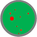
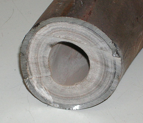
I have listed some of the data in the table as “Dynamic data but treated as static data.” This is because some data that are typically assumed to be fixed with time may, in fact, change. For example, the efficiency, absolute roughness, and relative roughness may change as the tubing degrades over time due to erosion, corrosion, or wax/asphaltene/scale deposition. I have also included the tubing/pipe diameter in this category of data because severe Scale Deposition (deposition of minerals from the produced water) can be a significant issue with certain produced water compositions and can significantly reduce the effective diameter of the tubing. This is shown in Figure 6.10. This figure also illustrates why tubing change-out workovers may be performed.
I have also highlighted some entries in Table 6.05 with blue cells (rows 7-9.) These entries are dynamic data that typically are not of interest to most production engineers and are not entered explicitly into a well model. These data are entered implicitly into the model by the choice of the multi-phase flow correlation selected by the engineer. I will discuss these dynamic data and these multi-phase flow correlations in more detail later in this lesson.
The table entries highlighted with orange cells (Table 6.05 rows 10-14) are entries with dynamic data that are of interest to the production engineers and are explicitly input into the well model. In actuality, only a subset of these data is required because the rates, , , and , are sufficient to specify the problem. For example, the oil rate, , the gas-oil ratio, , and water-oil ratio, , are sufficient to specify total production. Likewise, the liquid rate, , the gas-liquid ratio, , and watercut, , are also sufficient to specify total production.
Finally, the table entries highlighted with yellow cells (Table 6.05 rows 15-17) are entries that are either specified or calculated by the well model. As I mentioned earlier, as production engineers, we are typically concerned with two types of problems, Pressure Traverse Calculations, where we specify the flow rate and calculate the pressure drop, and Tubing Performance Calculations, where we specify one pressure and the total rate and calculate the other pressure (typically the flow bottom-hole pressure, ).
6.3.4.1: Multi-Phase Flow Correlations
As we have discussed, multi-phase flow through tubing is typically performed using empirical, multi-phase flow correlations. These empirical correlations are developed on the observations made by the investigator in laboratory experiments, field measurements, or both. The differences in the correlations are based on many factors including:
- experimental technique
- tubing orientation
- vertical
- slanted
- horizontal
- tubing type
- smooth
- rough
- fluids used in the experiments
- air-water
- crude oil - natural gas
- pressure-temperature range used in the experiments
- tubing orientation
- flow regimes observed during the experiments and how they are incorporated into the correlations
- trade-off between the desired accuracy and the desired degree of mathematical simplicity or ease of application
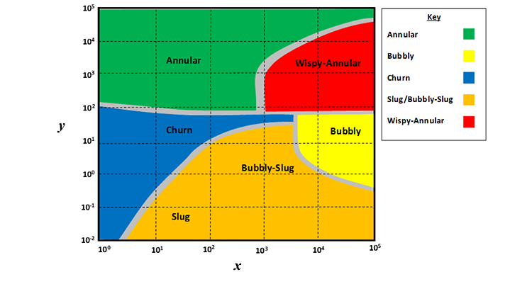
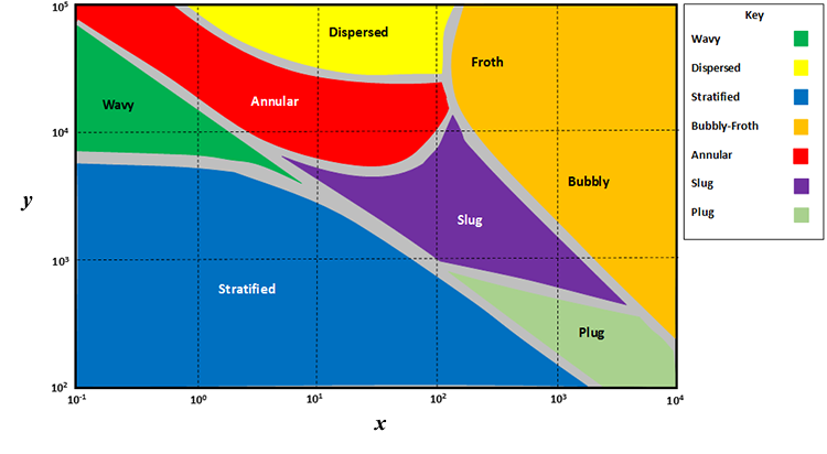
In most cases, the multi-phase flow correlations are based on the flow regimes that we have already discussed. For use in a multi-phase flow correlation, these flow regimes are plotted as Flow Pattern Maps. Examples of the flow pattern maps are shown in Figure 6.11 (for vertical flow) and Figure 6.12 (for horizontal flow).
Where: and
Where:
and
The example flow regime maps shown in Figure 6.11 and Figure 6.12 illustrate two important points. The first point is how the flow regimes are incorporated into the flow correlations. The variables on the x-axis and y-axis are calculated, and that point on the map indicates the flow regime that is occurring in a well segment based on the investigator’s experimental or field results. For the flow regime identified on the flow pattern map, different mathematical expressions are used to quantify the Liquid Hold-Up, Gas Hold-Up, the slip velocity, and the friction factors within that particular flow regime. These dynamic data are the data that I identified in Table 6.05 with the blue cells. Once the dynamic data are calculated for a particular segment in a segmented well model, they are used in the energy balance equation to determine the pressure loss in that segment.
The second point illustrated by the example flow pattern maps is that the definitions of the x-axis and y-axis are different for each multi-phase flow correlation. This gets back to the empirical nature of the multi-phase flow correlations. Different investigators and different experimental/field procedures may result in different mathematical groups controlling the dynamics of the flow. The choice of these mathematical groups may also lie in the personal preference of the investigator.
For multi-phase flow, the fluid properties are typically calculated as mixture properties. These mixture properties are based on the Phase Hold-Up, and . Hold-Up is the local fraction of the pipe volume occupied by the phase. In multi-phase flow correlations, the hold-up is determined from the map based on the mathematical expressions related to the flow regime. Once the hold-up is determined, fluid properties can be determined for the flowing mixture by:
for viscosity, some investigators prefer to use a different definition of mixture viscosity:
As a practical point, a working production engineer typically is not expected to know the details of the multi-phase flow correlation used in a well model. There is no universal rule for selecting the proper correlation for use for a particular well, group of wells, or wells in a field. The production engineer simply performs Flow Tests on his/her wells to see the actual pressure drops at the current reservoir conditions (orange and yellow table entries in Table 6.05) for known production rates and selects the multi-phase flow correlation that best matches the flow test results. Many software packages allow for the use of different multi-phase flow correlations for different segments of a segmented well model for one well. In other words, one well may use a different multi-phase flow correlation along different segments of the well.
Description of Multi-Phase Flow Correlations in Use in the Oil and Gas Industry
There are many multi-phase correlations used in the oil and gas industry. It is beyond the scope of this course to discuss all of the correlations in use today. Table 6.06 lists many of these correlations used in industry software along with notes describing their preferred applications.
| Single-Phase Flow |
Gas | Darcy-Weisbach | Theoretical Energy Balance. Uses a general friction factor. Requires an iteritive solution for copressible fluids. Can be used for wells (verticle, inclined, or horizontal), flow lines, or transmission lines. |
| Weymouth | Empiricla Energy Balance. Uses an equation specific friction factor. A non-iterative solutionis possible if inlet and outlet ressures are specified. An iterative solution is required otherwise. Can be used for wells, flow lines, or transmission lines. | ||
| Panhandle "A" | Empiricla Energy Balance. Uses an equation specific friction factor. A non-iterative solutionis possible if inlet and outlet ressures are specified. An iterative solution is required otherwise. Can be used for wells, flow lines, or transmission lines. | ||
| Panhandle "B" | Empiricla Energy Balance. Uses an equation specific friction factor. A non-iterative solutionis possible if inlet and outlet ressures are specified. An iterative solution is required otherwise. Can be used for wells, flow lines, or transmission lines. | ||
| Cullender and Smith | Empirical Energy Balance. Uses an equationspecific friction factor. Requires an iterative solution. | ||
| Liquid | Darcy-Weisbach | Theoretical Energy Balance. Uses a general friction factor. Requires an iterative solution for slightly compressible liquids. Can be used for wells (vertical, inclined, or horizontal), flow lines, or transmission lines. | |
| Hazen-Williams | Empirical. The friction factor is replaced with material specific constant. Requires an iterative solution for slightly compressible liquids. Used for water disposal, water source, water injection, or light hydrocarbon wells (possible use in condensate reservoirs). | ||
| Multi-Phase Flow |
Vertical Flow |
Fancher and Brown (no slip and no flow pattern map) |
The no slip assumption and no pattern map imply that the correlation is not generally applicable.The no slip assumption is only applicable in flow regimes where liquid and gas velocities are the same. |
|---|---|---|---|
| Hagedorn and Brown | Developed from experiments on 1,500 ft experimental well using 1 inch to 4 inch tubing. Experiments included thre-phase flow. One of the most commonly used multi-phase flow correlations for vertical or near vertical wells. | ||
| Beggs and Brill (no slip) |
The no slip assumption is only applicable in flow regimes where liquid and gas velocities are the same. One of the few multi-phase flow corrections capable of modeling vertical, inclined, or horizontal flow. Assumes smooth pipe. | ||
| Beggs and Brill (with Darcy-Weisbach friction factor) |
The no slip assumption is only applicable in flow regimes where liquid and gas velocities are the same. One of the few multi-phase flow corrections capable of modeling vertical, inclined, or horizontal flow. Pipe is allowed to include roughness. | ||
| Orkiszewski | Took existing correlations and compared them to field results. Selected the best correlations for different regimes and developed a single correlation. This is apopular multi-phase flow correlation, but may exhibit discontinuities when crossing regime boundaries. | ||
| Gray | Developed for gas condensate reservoirs (most accurate for these reservoirs). Uses non-compositional approach. It is based on the observation that hold-up is not as great in condensate wells as in oil wells. Roughness is ignored, but uses an efficiency instead. | ||
| Gray (with Darcy-Weiabach friction factor) |
Developed for gas condensate reservoirs (most accurate for these reservoirs). Similar to the standard Gray correlation, but roughness is incorporated through the Moody Diagram. | ||
| Duns and Ros | Uses combined experimental and field measurements. The first multi-phase flow correlation to use flow pattern mapping. A popular multi-phase flow correlation. | ||
| Horizontal Flow |
Eaton-Flanigan | This correlation is a hybrid correlation of the Eaton hold-up and friction loss correlations and the Flanigan inclined pipe correlation | |
| Eaton-Dunkler-Flanigan | This correlation is another hybrid correlation of the Eaton hold-up correlation, the Dukler friction correlation, and the Flanigan inclined pipe correlation. | ||
| Beggs and Brill (no slip) |
The no slip assumption is only applicable in flow regimes where liquid and gas velocities are the same. One of the few multi-phase flow correlations capable of modeling vertical, inclined, or horizontal flow. Assumes smooth pipe. | ||
| Beggs and Brill (with Darcy-Weisbach friction factor) |
The no slip assumption is only applicable in flow regimes where liquid and gas velocities are the same. One of the few multi-phase flow correlations capable of modeling vertical, inclined, or horizontal flow. Pipe is allowed to include roughness. |
6.3.4.2: Multi-Phase Flow Calculations
The analyses used for multi-phase flow are identical to those used for single-phase flow: pressure traverse calculations and tubing performance calculations. Figure 6.13 shows typical multi-phase pressure traverse plots using the Hagedorn and Brown Correlation. As seen in the legends of these plots, this figure indicates that the pressure drop is dependent on all of the properties listed in Table 6.05.
The difference in the pressure traverse curves shown in Figure 6.13, is the Watercut (fraction of water) in the produced stream: 0.0 for the family of curves on the left and 0.5 for the family of curves on the right. In these pressure traverse curves, the Static Properties (properties that are assumed to be constant over time) are the tubing I.D. the tubing lengths (TVD and MD), the oil API gravity, the gas specific gravity, and the water specific gravity; while the Dynamic Properties (properties that normally vary over time) are the wellhead pressure, the watercut , the gas/liquid ratio (GLR), and the production (liquid) rate. Other dynamic properties that are changing in the calculations include the flow regime, the hold-up, the local fluid (and mixture) properties, and friction factor.
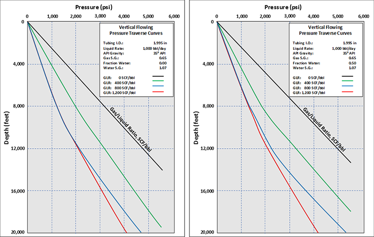
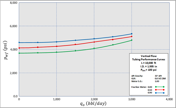
Figure 6.14 shows typical multi-phase tubing performance curves using the Hagedorn and Brown correlation. This figure shows a single, 10,000 ft tubing string with three different watercut values, 0.0, 0.5, and 0.9. The reason that the curve with the highest watercut (blue curve) has the highest flowing bottom-hole pressures, , is because water has a higher density than the oil which results in a heaver fluid column in the well. In the case of Figure 6.14, the 35º API crude oil has a specific gravity of 0.85, while the water has a specific gravity of 1.0.
6.4: Key Learnings
- Three common well orientations for crude oil and natural gas production are vertical wells, deviated (or slanted) wells, and horizontal wells. These wells have different applications in field development, but all can be modeled with contemporary well modeling software.
- Tubing hydraulics during crude oil and natural gas production is a very complex physical problem, particularly for multi-phase flow. These parameters that impact tubing hydraulics include:
- the well design: well orientation and tubing size
- the well condition: absolute and relative roughness
- the production rate: dependent on reservoir inflow performance
- number and types of flowing phases: this will change based on:
- the location of the fluids in the well (with respect to the local bubble-point pressure)
- pressure depletion in the reservoir
- the fluid properties: density, viscosity, etc.
- the local flow regimes in the segment tubing:
- laminar or turbulent
- multi-phase flow regimes illustrated in Table 6.01 and Table 6.02
- Fluids flowing through tubing do not flow as homogeneous fluids but may go through many flow regimes or flow patterns:
- for vertical flow:
- single-phase flow
- bubble flow
- slug flow
- churn flow
- annular flow
- mist flow
- for horizontal flow:
- single-phase flow
- bubble flow
- plug flow
- stratified flow
- wavy flow
- slug flow
- annular flow
- spray flow
- for vertical flow:
- The well does not necessarily need to pass through all of these flow regimes. The flow patterns can be quantified for numerical calculations with flow pattern maps. Flow regime maps are empirically based maps that indicate the flow regime at know pipe/tubing conditions (x-axis and y-axis on the flow pattern map).
- The fundamental relationship for tubing hydraulics is the energy equation developed by Bernoulli.
- The energy balance equation that was specifically adapted from Bernoulli’s equation for pipe/tubing flow is the Darcy-Weisbach Equation. The Darcy-Weisbach Equation can be used for all single-phase flow conditions. Friction losses in well tubing are calculated with Darcy-Weisbach Friction Factor. The Darcy-Weisbach Friction Factor is plotted in the Moody Diagram as a function of the Reynolds Number and the relative roughness of the pipe/tubing.
- Other empirical single- phase flow correlations can be used for tubing hydraulics:
- liquids: the Hazen-Williams Equation for water and light hydrocarbons
- gases: the Weymouth equation, the Panhandle “A” equation, and the Panhandle “B” equation
- There are two main types of tubing hydraulics calculations used by Production Engineers: Pressure Traverse Calculations and Tubing Performance Calculations. Pressure traverse calculations are based on a known flow rate, , and an unknown pressure drop, . Tubing performance calculations are based on a known flow rate, , a known wellhead pressure, , and an unknown flowing bottom-hole pressure, .
- For multi-phase flow, the flow problem is too complex to solve theoretically, and empirical flow correlations based on the flow patterns maps are used. The flow pattern maps have empirical correlations for hold-up, slip, and friction for the different flow regimes observed in laboratory and field experiments. These correlations are used in the energy balance equation to perform tubing hydraulics calculations. The multi-phase correlations currently in use in the oil and gas industry include:
- Verical flow:
- Fancher and Brown
- Hagedorn and Brown
- Beggs and Brill
- Orkiszewski
- Gray
- Duns and Ros
- Horizontal and deviated flow:
- Eaton-Flanigan
- Eaton-Dukler-Flanigan
- Beggs and Brill
- Verical flow:
6.5: Summary and Final Tasks
Summary
In this lesson, we discussed a very important task performed by production engineers working on crude oil and natural gas production wells. This task is to calculate the pressure drop in well tubing. As we will see, this is a very powerful tool for helping production engineers design and optimize production and injection wells. In addition to aiding in the initial well design, these analyses help in decisions on improving well performance, such as, adding artificial lift (gas lift or pump) to the well, stimulating the well (hydraulic fracture or acidation), and other workovers and well interventions.
In this lesson, we discussed the basics of tubing hydraulics related to oil and gas production. The well hydraulics are governed by an energy balance that relates the pressure, velocity, and elevation of a flowing fluid to its potential energy and frictional losses. The resulting equation, the Darcy-Weisbach Equation, related the rate flowing through the pipe/tubing to the pressure drop in the tubing.
For single-phase flow, the flow problem can be solved with theoretical considerations, while for multi-phase flow empirical correlations are used. These multi-phase flow correlations are based on flow pattern maps which enable different mathematical descriptions of dynamic two-phase data (such as, hold-up, slip velocity, and frictional losses) in different flow regimes. For selection of the appropriate correlation, production engineers reply on flow tests to assess the accuracy of the different flow correlations and to calibrate these correlations to their wells.
Final Tasks
Complete all of the Lesson 6 tasks!
You have reached the end of Lesson 6! Double-check the to-do list on the Lesson 6 Overview page [17] to make sure you have completed all of the activities listed there before you begin Lesson 7.