6.3.1: Equations Governing Flow in Pipe and Tubing

Bernoulli’s Equation

Bernoulli’s Equation forms the basis of the steady-state tubing performance. Bernoulli’s Equation is simply an energy balance on a given system. In our case, that system is the production tubing. Bernoulli’s Equation can be written as:

In this equation, all of the terms have the units of lb_f-ft. The variables in this equation are:

• $U_1$ and $U_2$ are the Internal Energies stored in the fluid at two points in the system, lb_f-ft. This internal energy is energy at the molecular level and cannot be measured in an absolute sense. We can establish the relative change in the internal energy ($\Delta U=U_1-U_2$) by assigning a zero value at some specific set conditions.
• $p_1$ and $p_2$ are the pressures at two points in the system, psi
• $V_1$ and $V_2$ are the volumes of the fluid at two points in the system, ft³
• The terms $\frac{p_1{V}_1}{144}$ and $\frac{p_2{V}_2}{144}$ are the Energies of Expansion or Compression, lb_f-ft. These terms represent compressional energy stored in the fluid (similar to the energy stored in a compressed spring).
• $m$ is the mass of the fluid in the system, lb_m
• $v_1$ and $v_2$ are the velocities of the fluid at two points in the system, ft/sec
• $g_c$ is the Universal Gravitational Constant, 32.174 lb_m-ft/lb_f-sec²
• The terms $\frac{m{v}_1^2}{2g_c}$ and $\frac{m{v}_2^2}{2g_c}$ are the Kinetic Energy of the fluid in the system, lb_f-ft
• $g$ is the Local Acceleration due to gravity, ft/sec². The local acceleration due to gravity varies from location to location but is approximately equal to 32.174 ft/sec². The ratio of $\frac{g}{g_c}$ is approximately equal to 1.0 lb_f/lb_m.
• $z_1$ and $z_2$ are elevations above some reference point, typically sea level, ft
• The terms $\frac{mg{z}_1}{g_c}$ and $\frac{mg{z}_2}{g_c}$ are the Potential Energies of the fluid at two points in the system, lb_f-ft
• $Q_H$ is the Thermal Energy added to or removed from the system, lb_f-ft. In Equation 6.01, $Q_H$ is positive if thermal energy is added to the system or negative if thermal energy is removed from the system (note: 1 BTU = 778.169 lb_f-ft)
• $W$ is the work added to or performed by the fluid, lb_f-ft. In Equation 6.01, $Q_H$ is positive if work is added to the system (for example, with a pump) or negative if work is removed from the system (for example, by turning a turbine)

There are many engineering Thermodynamics concepts in this equation which are out-of-scope for this course; however, we can illustrate the application of Bernoulli’s Equation in the context of flow through tubing with Figure 6.04.

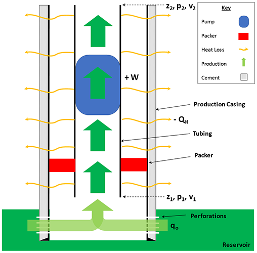
In Figure 6.04, we have a length of vertical tubing defined from a depth of $z_1$ to a depth of $z_2$ with an inner diameter of $D_{ID}$. A mass of oil enters the tubing at $z_1$ at a volumetric rate of $q$ (ft³/sec) at a pressure of $p_1$ and a velocity of $v_1=\frac{q}{A}\frac{4q}{\pi D_{ID}^2}$. As the oil travels up from the reservoir, the surrounding rock is cooler than the oil due to the local geothermal gradient, and heat is lost ($-Q_H$) from the hot oil to the surrounding cooler rock. Flowing upward, the oil encounters a downhole pump which supplies work ($+W$) to the system. The oil finally reaches point $z_2$ in the tubing with a Terminal Pressure of $p_2$ and Terminal Velocity of $v_2$.

Without going into the thermodynamic details, Equation 6.01 can be rewritten in differential form as:

Where:

and,

• $p$ is the pressure at a point in the tubing, psi
• $l$ is the distance along the axis of the tubing, ft
• 144 is a unit conversion constant, in²/ft²
• 12 is a unit conversion constant, in/ft
• $g_c$ is the Universal Gravitational Constant, 32.174 lb_m-ft/lb_f-sec²
• $g$ is the Local Acceleration due to gravity, ft/sec². The local acceleration due to gravity varies from location to location but is approximately 32.174 ft/sec². The ratio of $\frac{g}{g_c}$ is approximately 1.0 lb_f/lb_m
• $\theta$ is the angle of inclination above the horizontal, dimensionless
• $f_{DW}$ is the Darcy-Weisbach Friction Factor, dimensionless
• $v$ is the velocity of the fluid at the point in the tubing, ft/sec
• $\rho$ is the density of the fluid, lb_m/ft³
• $D_{ID}$ is the Inner Diameter ($ID$) of the tubing, in
• $z$ is the elevation of the point in the tubing above a reference point, typically sea level, ft

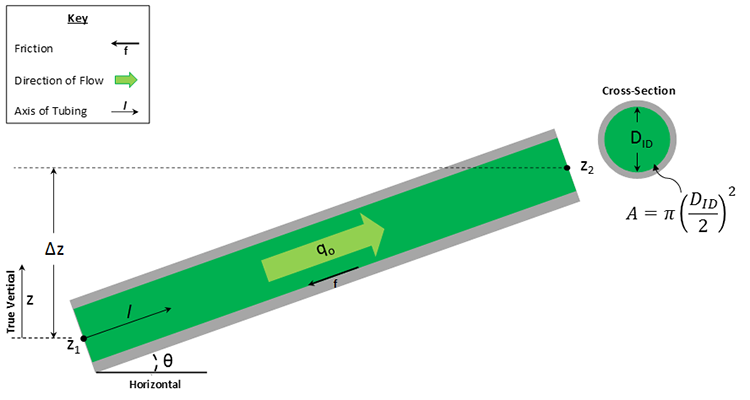
The units of each of the terms in Equation 6.02 and Equation 6.03 are psi/ft. The well orientation for Equation 6.02 and Equation 6.03 is shown in Figure 6.05.

In Equation 6.02, I have neglected the Heat Transfer, $Q_H$, and Work, $W$, terms. If we have significant heat transfer or a device that adds or performs work, we can include these terms into the equation.

Expanding on the terms in Equation 6.02, the elevation term, ${\left(\frac{dp}{dl}\right)}_{Elevation}$, is simply the change in the potential energy as the fluid flows through the tubing in the direction of $l$. Note that in the convention shown in Figure 6.05 with the z-direction upward, point $z_2$ has a higher potential energy than point $z_1$ because it has a higher elevation. The friction term, ${\left(\frac{dp}{dl}\right)}_{Friction}$, is the irreversible loss of energy due to friction as the fluid flows past the stationary tubing wall. Friction always acts in the direction of opposite of flow. For single-phase flow, the only friction component occurs at the liquid-tubing interface. In multi-phase flow where phases are flowing at different velocities, there will be a friction component occurring at the phase boundaries also. Finally, the acceleration term, ${\left(\frac{dp}{dl}\right)}_{Acceleration}$, is the change in energy resulting from the acceleration or deceleration of the fluid going around bends in the tubing. The acceleration term is often neglected in tubing calculations.

As mentioned earlier, the friction factor, fDW, in Equation 6.03b is the Darcy-Weisbach friction factor. This equation is co-credited to Henry Darcy, who is the same Darcy that gave us Darcy’s Law. The Darcy-Weisbach friction factor is the ratio of the shear stress at the wall and the kinetic energy of the fluid on a unit volume basis. This friction factor was plotted by Moody^[1]as a function of the Reynolds Number^[2],[3], ${\mathrm{R}}_e$, and the Relative Roughness $\left(\frac{\epsilon }{D_{ID}}\right)$. The Moody Diagram is shown in Figure 6.06.

Note, we will be using the Darcy-Weisbach friction factor, $f_{DW}$, which is not to be confused with the Fanning Friction Factor, $f_F$^[4]. The Fanning friction factor is ¼ the value of the Darcy-Weisbach friction factor, that is: $f_F=\frac{1}{4}{f}_{DW}$. The difference between the two friction factors is that the Darcy-Weisbach friction factor is typically used for closed circular pipes, and uses $D_{ID}$ as the diameter, while the Fanning friction factor can be used for open conduits and uses the concept of the “hydraulic radius” as a measure of the diameter: $r_h=\frac{A}{p}$. Where $r_h$ is the hydraulic radius, $A$ is the cross-sectional area of flow (length squared), and $P$ is the “wetted perimeter” (length). The wetted perimeter is the perimeter of the cross-section in contact with the conduit (portion of the cross-section that is “wetted” by the fluid).

The Reynolds Number, ${\mathrm{R}}_e$, is a dimensionless group that represents the ratio of the inertial forces to the viscous forces within the fluid and is used to characterize laminar and turbulent flow regimes. For our application of flow through pipe, the Reynolds Number is defined by:

Where:

• $N_{RE}$ is the Reynolds Number, dimensionless
• 1488.0 is a unit conversion constant, ft-sec-cp/lb_m
• 12 is a unit conversion constant, in/ft
• 124 in an equation constant
• $D_{ID}$ is the Inner Diameter ($ID$ ) of the tubing, in
• $v$ is the velocity of the fluid in the tubing, ft/sec
• $\rho$ is the density of the fluid, lb_m/ft³
• $\mu$ is the dynamic viscosity of the fluid, cp

Note, Equation 6.04a can be expressed in an equivalent form in terms of flow rate, $q\left(bbl/day\right)$:

Where the velocity term was replaced with the rate term: $v\left(\frac{ft}{\sec }\right)=\frac{q}{A}=\frac{\left(4\right)144\left(\frac{i{n}^2}{f{t}^2}\right)}{\pi D_{ID}^2\left(i{n}^2\right)}\frac{5.615\left(\frac{f{t}^3}{bbl}\right)q\left(\frac{bbl}{day}\right)}{24\left(\frac{hr}{day}\right)60\left(\frac{\min }{hr}\right)60\left(\frac{\sec }{\min }\right)}$.

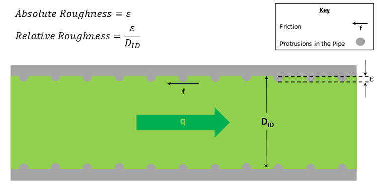
At lower values of ${\mathrm{R}}_e$ $\left({\mathrm{R}}_e<2,000\right)$ flow is in the laminar flow regime, while at higher values of ${\mathrm{R}}_e$ $\left({\mathrm{R}}_e>4,000\right)$ flow is in the turbulent flow regime. As we see in the Moody Diagram, Figure 6.06, in the turbulent flow regime the friction factor is a function of the Reynolds Number and relative roughness of the pipe $\left(\frac{\epsilon }{D_{ID}}\right)$. The relative roughness is a dimensionless quantity that is defined as the length of protrusions (lumps, pipe defects and imperfections, pits from corrosion, etc.) divided by the inner diameter of the tubing. It is a measure of the departure of an actual steel pipe from an idealized, smooth pipe. Figure 6.07 illustrates the concepts of absolute and relative roughness, while Table 6.03 shows typical values of the absolute roughness, $\epsilon$, for different materials.

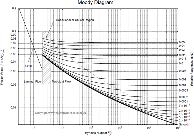
In the laminar flow regime $\left({\mathrm{R}}_e<2,000\right)$, the Darcy-Weisbach friction factor is a function of the Reynolds Number only and can be determined by:

Table 6.03: Typical Values of the Absolute Roughness, $\epsilon$^[5]

Material	$\epsilon (mm)$	$\epsilon (in)$
Idealized smooth surface – any material	0.0	0.0
Concrete – coarse	0.2500	0.009842
Concrete – new smooth	0.0250	0.000984
Drawn tubing	0.0025	0.000098
Glass, Plastic Perspex	0.0025	0.000098
Iron – cast	0.1500	0.005906
Sewers – old	3.0000	0.118110
Steel – mortar lined	0.1000	0.003937
Steel – rusted	0.5000	0.019685
Steel – structural or forged	0.2500	0.009842
Water mains – old	1.0000	0.039370

As previously discussed, in the turbulent flow regime, the Darcy-Weisbach friction factor is a function of both the Reynolds Number and the relative roughness. To calculate the friction factor in the turbulent regime, the Implicit Colebrook Equation^[6] can be used:

We say that this equation is implicit because the friction factor, $f_{DW}$, appears on both sides of the equals sign. Therefore, to solve this equation, we must iterate on a solution. That is, we make an initial guess at $f_{DW}$ and use it on the right-hand side of the equation to calculate a new $f_{DW}$ on the left-hand side of the equation. We repeat this process until the two values of $f_{DW}$ (the recently calculated value on the left-hand side of the equation and the value used in the calculation on the right-hand side of the equation) are sufficiently close. To start the process, an Explicit Formula for $f_{DW}$, such as the Swamee-Jain Equation^[7], is used:

We say that Equation 6.07 is an explicit formula because the friction factor does nor appear on the right-hand side of the equation, and we can solve for it explicitly. The Swamee-Jain Equation^[7] is an approximation to the Colebrook Equation^[6] and can also be used directly in calculations.

---