Well Modeling
Well Modeling is the process of developing models (supplying input) for actual wells and using these data in Well Modeling Software to perform the analyses required by the engineer. In all of our discussions to this point, we have assumed single-phase flow of either liquid or gas. Pressure loss calculations in multi-phase flow are much more complicated than those for single-phase flow. This is because in single-phase flow, the only frictional losses that occur in the system are at the fluid-pipe interface. In multi-phase flow, there is also the friction loss between the phases. As we have also seen in our discussion on flow regimes in tubing, there are multiple flow regimes that can occur in vertical, deviated, and horizontal wells and these can have a significant impact of energy and momentum transfer.
To quantify the pressure losses occurring in multi-phase flow calculations, we must consider the physics that are occurring in each flow regime. Typically, in the oil and gas industry, for multi-phase flow we evaluate the physics empirically. Table 6.05 lists the important physical data that have been observed to have a significant impact on the pressure drop in well tubing. These empirical physics are input into the well model with a Multi-Phase Flow Correlation.
There are many multi-phase flow correlations available and most pipe flow or nodal analysis software contains options for the most relevant correlations for crude oil and natural gas flow. The details of these multi-phase flow correlations are beyond the scope of this class, so I will briefly give a general description of them and then discuss the common correlations used in the oil and gas industry.
Well Model Data
As we have already discussed, the energy balance is a steady-state equation while our flow calculations are unsteady-state problems. When we use the energy balance equation to solve unsteady-state problems, we are solving a category of physical problems called a Series of Steady-States where the equation is derived for steady-state conditions, but we are solving it with time-dependent input data.
In Table 6.05 there are color coded entries: some of the data I have listed as Static Data which implies they do not change with time or location. Other data I have listed as Dynamic Data which implies that they may change with time, location, or both.
The entries in the green cells (Table 6.05 rows 1-6) are the data that make up a Well Model. These data are entered into the well modeling software and are treated as fixed data for some time period or some length of tubing. For example, I have already mentioned tapered tubing strings where the diameter of the tubing may change with position. When a well model is constructed, these design changes can be implemented as part of the segmented well model.
| Data or Property | Symbol | Description |
|---|---|---|
| Tubing/Pipe Diameter | Dynamic data but treated as static data | |
| Downhole well equipment | Pumps, chokes, etc. | Static data |
| True vertical depth, TVD | Vertical depth – depth in the true vertical direction | |
| Measured depth, MD | Measured depth – physical length of tubing | |
| Absolute or Relative Roughness | Dynamic data but treated as static data | |
| Efficiency | Dynamic data but treated as static data | |
| Liquid Hold-Up | Dynamic data: fraction of a representative elemental volume (REV) occupied by liquid (analogous to liquid saturation in the reservoir). | |
| Gas Hold-Up | Dynamic data: fraction of a representative elemental volume (REV) occupied by gas (analogous to gas saturation in the reservoir). | |
| Slip (or Slip Velocity) | Dynamic data (difference between velocities of two different phases). | |
| Gas-Liquid Ratio | Dynamic data: used as input to our pressure traverse or tubing performance calculation. | |
| Gas-Oil Ratio or | Dynamic data: used as input to our pressure traverse or tubing performance calculation. | |
| Watercut or | Dynamic data: fraction of the water rate in the total liquid rate. Used as input to our pressure traverse or tubing performance calculation. | |
| Water-Oil Ratio or | Dynamic data: ratio of the water water rate to the oil rate. Used as input to our pressure traverse or tubing performance calculation. | |
| Oil, Gas, and Water PVT Properties | Dynamic data: Pressure-Volume-Temperature description of all fluids. | |
| Well Head Pressure | Dynamic data: one of the primary knowns/unknowns of the problem. | |
| Bottom-Hole Pressure | Dynamic data: one of the primary knowns/unknowns of the problem:
|
|
| Production/Injection Rate | Dynamic data: one of the primary knowns/unknowns of the problem. |
Static data may also change due to a well intervention. For example, a production engineer may decide to perform a Tubing Change-Out Workover, where all or portions of the tubing string are removed from the well and replaced with new tubing (either the original size or a new size). When a new tubing string is used, or a new piece of downhole equipment is installed, this is considered a new well design, and a new model must be used.
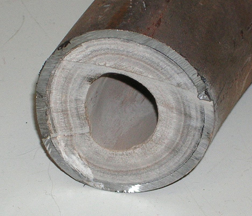
I have listed some of the data in the table as “Dynamic data but treated as static data.” This is because some data that are typically assumed to be fixed with time may, in fact, change. For example, the efficiency, absolute roughness, and relative roughness may change as the tubing degrades over time due to erosion, corrosion, or wax/asphaltene/scale deposition. I have also included the tubing/pipe diameter in this category of data because severe Scale Deposition (deposition of minerals from the produced water) can be a significant issue with certain produced water compositions and can significantly reduce the effective diameter of the tubing. This is shown in Figure 6.10. This figure also illustrates why tubing change-out workovers may be performed.
I have also highlighted some entries in Table 6.05 with blue cells (rows 7-9.) These entries are dynamic data that typically are not of interest to most production engineers and are not entered explicitly into a well model. These data are entered implicitly into the model by the choice of the multi-phase flow correlation selected by the engineer. I will discuss these dynamic data and these multi-phase flow correlations in more detail later in this lesson.
The table entries highlighted with orange cells (Table 6.05 rows 10-14) are entries with dynamic data that are of interest to the production engineers and are explicitly input into the well model. In actuality, only a subset of these data is required because the rates, , , and , are sufficient to specify the problem. For example, the oil rate, , the gas-oil ratio, , and water-oil ratio, , are sufficient to specify total production. Likewise, the liquid rate, , the gas-liquid ratio, , and watercut, , are also sufficient to specify total production.
Finally, the table entries highlighted with yellow cells (Table 6.05 rows 15-17) are entries that are either specified or calculated by the well model. As I mentioned earlier, as production engineers, we are typically concerned with two types of problems, Pressure Traverse Calculations, where we specify the flow rate and calculate the pressure drop, and Tubing Performance Calculations, where we specify one pressure and the total rate and calculate the other pressure (typically the flow bottom-hole pressure, ).