GEOG 586
Geographic Information Analysis

Project 7: Allocation Based on Straight-Line Distance

PrintPrint

Note:

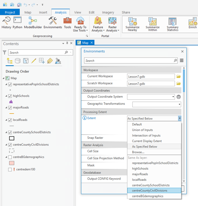
Analysis - Environments...should be set appropriately before doing any analysis (Figure 7.5).

In particular, use the centreCountyCivilDivisions layer as the Mask and also for the Processing Extent. You should also carefully consider what is an appropriate Cell Size for the analysis and set that parameter.

Screenshot of how to set analysis environment
Figure 7.5: Setting Analysis Environments. 
Click for a text description of the Setting Analysis Environments image.
Both the Mask and Processing Extent should be set to centreCountyCivilDivisions in the Analysis Environment window.
Credit: Griffin, 2019

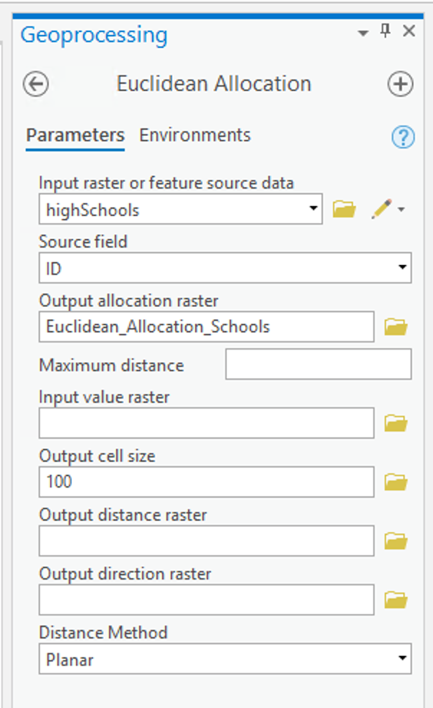
The first analysis we will do uses the Spatial Analyst Tools - Distance - Euclidean Allocation tool from the Tools menu (Figure 7.6). This allocates each part of the map to the closest one of a set of points and is the raster equivalent of proximity polygons.

Euclidean Allocation tool with parameters set in the fields.
Figure 7.6: The Euclidean Allocation user interface with parameters set to generate an allocation of areas to high schools.
Click for a text description of the Euclidean Allocation user interface image.
The input features parameter should be set to the high schools layer. The source field should be set to ID. Name the output allocation layer something sensible, such as Euclidean_Allocation_Schools. Be sure that you save your output layer to the gdb and not another folder. If one of the schools has no cells allocated to it, you've likely saved the output outside the gdb. The cell size will be autopopulated with the value you set for cell size in the Analysis Environments settings dialogue.
Credit: Griffin, 2019

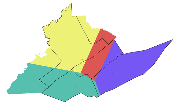
Running this Euclidean Allocation (straight line distance) analysis will produce an allocation layer (Figure 7.7).

Allocation layer
Figure 7.7: Allocation layer created from the Euclidean Allocation analysis.
Click for a text description of the Euclidean Allocation analysis output image.
This image shows the output of the Euclidean Allocation analysis with the settings described in the lesson. There is a mismatch in alignment between the allocation areas generated by the tool and the actual school districts. The allocation districts are most poorly aligned in areas that contain mountain ridges.
Credit: Griffin, 2019

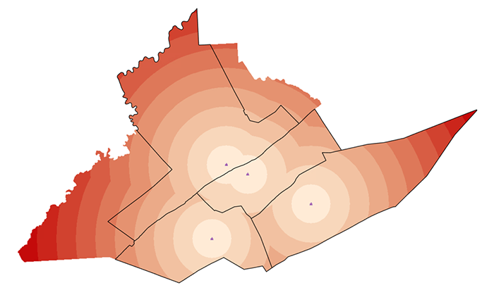
You can also request a distance layer (Figure 7.8).

Distance layer
Figure 7.8: Results of the Euclidean Distance analysis for high schools.
Click for a text description of the Euclidean Distance analysis outputs image.
In the Euclidean Distance analysis output, the raster cells contain values that describe the distance to the nearest school. The image looks like concentric buffer rings whose overlaps have been dissolved.
Credit: Griffin, 2019

You can further analyze these layers. For example, it may be easier to read the distance analysis if you create contour lines. The results of the allocation analysis can be converted to vector polygons, which might make subsequent analysis operations easier to perform, depending on which approach you decide to take.

Deliverable

In your Project 7 write-up, describe how the distance analysis operation works. In your description, comment on how you would combine multiple distance analysis results (one for each high school) to produce an allocation analysis output. [Hint: First run the Euclidean Distance Tool for each high school individually and then look for a tool that when used can generate the same map that the Euclidean Allocation analysis provides (i.e., the map shown in Figure 7.7). There is a tool which could help with this -- take a look at the tools available in Spatial Analyst - Local (e.g., Cell statistics or Lowest).]

As part of your discussion, include the output maps generated by the Euclidean Allocation and Euclidean Distance processes.

Finally, comment on the differences in the Euclidean (straight-line) distance allocation and the actual allocation of places to school districts. (You will need to look at the roads, topography, and minor civil divisions to make sense of this.)