Like the nominal level of measurement, ordinal scaling assigns observations to discrete categories. Ordinal categories are ranked, however. It was stated in the preceding page that nominal categories such as "woods" and "mangrove" do not take precedence over one another unless an extrinsic set of priorities is imposed upon them. In fact, the act of prioritizing nominal categories transforms nominal level measurements to the ordinal level.
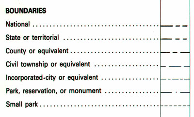
Examples of ordinal data often seen on reference maps include political boundaries that are classified hierarchically (national, state, county, etc.) and transportation routes (primary highway, secondary highway, light-duty road, unimproved road). Ordinal data measured by the Census Bureau include how well individuals speak English (very well, well, not well, not at all), and level of educational attainment. Social surveys of preferences and perceptions are also usually scaled ordinally.
Individual observations measured at the ordinal level typically should not be added, subtracted, multiplied, or divided. For example, suppose two 640-acre grid cells within your county are being evaluated as potential sites for a hazardous waste dump. Say the two areas are evaluated on three suitability criteria, each ranked on a 0 to 3 ordinal scale, such that 0 = unsuitable, 1 = marginally unsuitable, 2 = marginally suitable, and 3 = suitable. Now say Area A is ranked 0, 3, and 3 on the three criteria, while Area B is ranked 2, 2, and 2. If the Siting Commission was to simply add the three criteria, the two areas would seem equally suitable (0 + 3 + 3 = 6 = 2 + 2 + 2), even though a ranking of 0 on one criterion ought to disqualify Area A.