DEMs are produced by various methods. The method preferred by USGS is to interpolate elevations grids from the hypsography and hydrography layers of Digital Line Graphs.
The elevation points in DLG hypsography files are not regularly spaced. DEMs need to be regularly spaced to support the slope, gradient, and volume calculations they are often used for. Grid point elevations must be interpolated from neighboring elevation points. In Figure 7.9.2 for example, the gridded elevations shown in purple were interpolated from the irregularly spaced spot elevations shown in red.
Here's another example of interpolation for mapping. The map below in Figure 7.9.3 shows how 1995 average surface air temperature differed from the average temperature over a 30-year baseline period (1951-1980). The temperature anomalies are depicted for grid cells that cover 3° longitude by 2.5° latitude.
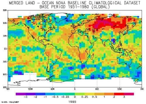
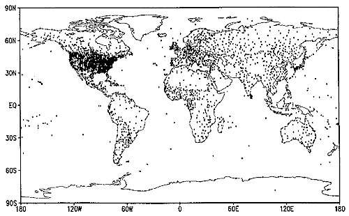
The gridded data shown above were estimated from the temperature records associated with the very irregular array of 3,467 locations pinpointed in the map below. The irregular array is transformed into a regular array through interpolation. In general, interpolation is the process of estimating an unknown value from neighboring known values.
Elevation data are often not measured at evenly-spaced locations. Photogrammetrists typically take more measurements where the terrain varies the most. They refer to the dense clusters of measurements they take as "mass points." Topographic maps (and their derivatives, DLGs) are another rich source of elevation data. Elevations can be measured from contour lines, but obviously, contours do not form evenly-spaced grids. Both methods give rise to the need for interpolation.
The illustration above shows three number lines, each of which ranges in value from 0 to 10. If you were asked to interpolate the value of the tick mark labeled "?" on the top number line, what would you guess? An estimate of "5" is reasonable, provided that the values between 0 and 10 increase at a constant rate. If the values increase at a geometric rate, the actual value of "?" could be quite different, as illustrated in the bottom number line. The validity of an interpolated value depends, therefore, on the validity of our assumptions about the nature of the underlying surface.
As I mentioned in Chapter 1, the surface of the Earth is characterized by a property called spatial dependence. Nearby locations are more likely to have similar elevations than are distant locations. Spatial dependence allows us to assume that it's valid to estimate elevation values by interpolation.
Many interpolation algorithms have been developed. One of the simplest and most widely used (although often not the best) is the inverse distance weighted algorithm. Thanks to the property of spatial dependence, we can assume that estimated elevations are more similar to nearby elevations than to distant elevations. The inverse distance weighted algorithm estimates the value z of a point P as a function of the z-values of the nearest n points. The more distant a point, the less it influences the estimate.
The illustration shows how the elevation of a given point P can be estimated by averaging the known elevations of nearby points, while taking into account their distance from point P. The fancy technical term for the procedure is "inverse distance weighted interpolation."