4.4.1.3: Steady-State Flow of Oil to a Vertical Production Well in Terms of the Average Pressure

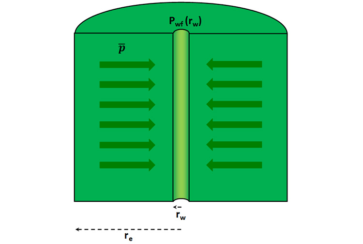
In our earlier discussions, we used the pressure drop from the external radius, $p_e$ at $r_e$ to determine the production rate, $q$. In many situations, we may not know the reservoir pressure at $r_e$; however, we may know the average reservoir pressure, $\overline{p}$. In fact, as we will see during our discussion on material balance, this is actually the more common situation. This situation is depicted in Figure 4.04, where the pressure at the external radius, $p_e\left(r_e\right)$ has been replaced with the average pressure, $\overline{p}$, in the interior of the drainage volume.

We can also develop equations for production rate for cases where we only know $\overline{p}$. To do this, we start with Equation 4.12. Rather than integrating this equation from $r_w$ to $r_e$, we can change the limits of integration from $r_w$ to an arbitrary radius, $r$, and the corresponding pressure at this radius, $p$:

This results in an equation similar to Equation 4.14, but incorporating the arbitrary integration limits:

Solving for the pressure, $p$, results in:

Equation 4.25 describes the Pressure Distribution (pressure as a function of location, which in our case is the pressure as a function radius) in the drainage volume. As one would expect, this equation indicates that as the radius, $r$, increases away from the production well, the pressure also increases (i.e., fluids are flowing from regions of high pressure to the region of low pressure, the production well). The volumetric average of any property, $P$ (where upper case “$P$” is any point-by-point property), can be calculated from:

Now, the volume of a cylinder is defined as:

Differentiating Equation 4.27 with respect to volume assuming a uniform thickness, $h$ , results in:

Substituting Equation 4.27 and Equation 4.28 into Equation 4.26 yields:

Now, substituting Equation 4.25 into Equation 4.29:

Performing the integration yields:

or,

or,

If we assume that $r_e>>r_w$, then $\frac{r_e{}^2}{r_e{}^2-r_w{}^2}\approx 1$. This is a very good assumption because the radius of the drainage volume of a well is typically on the order of hundreds or thousands of feet while the radius of the well is normally less than one foot. Using this approximation, Equation 4.31c becomes:

or, after rearranging:

Using the same methodology discussed earlier, we can also introduce the skin factor, $S$, to account for well damage or stimulation:

Equation 4.34 is the relationship between the production rate of a liquid, $q$, and the average reservoir pressure, $\overline{p}$. This equation has a similar form to that of Equation 4.19, but with two notable differences:

• The factor of ½ in the denominator of Equation 4.34
• The use of the average reservoir pressure in the drainage volume, $\overline{p}$, the pressure drop calculation in Equation 4.34

As I mentioned earlier, the use of, $\overline{p}$, has important consequences when applying material balance methods. We will discuss this later in this lesson.