4.4.1.4: Pseudo Steady-State Flow of Oil to a Vertical Production well

In all of our discussions on well performance, we assumed that Steady-State Conditions (time-invariant conditions) were occurring in the reservoir. Steady-state implies that nothing changes in the drainage volume with time or production. This simplification is not appropriate for most real production situations. Figure 4.05 shows the more common Transient Flow Conditions (time-dependent conditions) that occurs in the reservoir.

Figure 4.05: Pressure Distributions as a Function of Time

Source: Greg King

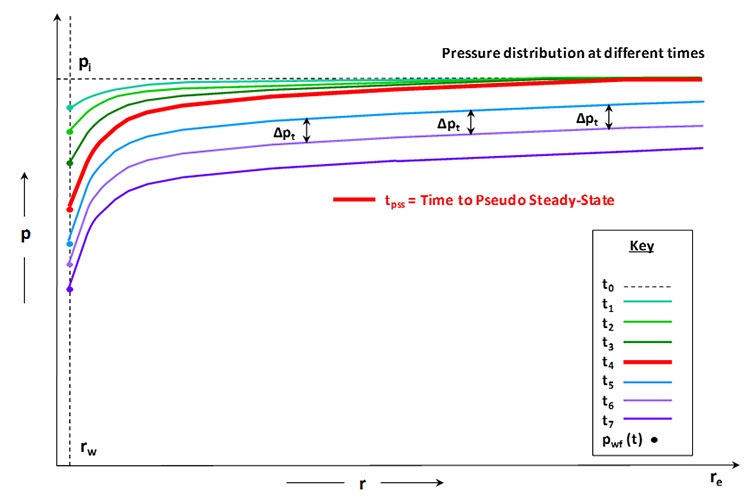
In this figure, the early-time pressures (green curves) form a pressure disturbance that over time propagates outward toward the external radius of the drainage volume, $r_e$. At some point in time, this pressure disturbance reaches the external boundary (bold red curve). This time is referred to as the time to pseudo steady-state, $t_{pss}$. Pseudo steady-state is a flow regime which is defined by a uniform pressure drop from one time to the next, $\Delta p_t$, that is equal everywhere in the drainage volume. This is illustrated in Figure 4.05 by the blue curves. The solid dual-headed arrows indicate that the pressure drop is the same at each radius in the reservoir.

The transient behavior of a radial-cylindrical drainage volume with uniform (constant) reservoir properties is governed by the partial differential equation (diffusivity equation):

I will derive this equation later in the lesson when we discuss fully transient flow; however, for the time being, we will consider its use in the context of pseudo steady-state flow. Without going into the details, the solution to this equation at times greater than $t_{pss}$ can be approximated by:

Where:

• 5.615 is a unit conversion constant, ft³/bbl
• 1.127x10^-3, 141.22, and 0.012648 are equation constants
• $p_{wf}$ is the flowing well pressure, psi
• $p_i$ is the initial reservoir pressure, psi
• $\mu$ is viscosity, cp
• $B$ is the formation volume factor, bbl/STB
• $q$ is the liquid rate in STB/day
• $k$ is the permeability, md
• $h$ is the reservoir thickness, ft
• $t$ is the time, days
• $\varphi$ is the porosity of the reservoir, fraction
• $c_t$ is total compressibility of the system, 1/psi
• $r_e$ is the external radius of the drainage volume, ft
• $r_w$ is the well radius, ft

Now, for slightly compressible liquids, we can calculate the average reservoir pressure by using the definition of compressibility:

In Equation 4.37, we set $\Delta V$ equal to the volume produced from the well over the time period $t$, $\Delta V\left(f{t}^3\right)=5.615qtB\left(f{t}^3\right)$, and $V$ equal to the pore volume of the drainage volume in ft³. Substituting $p_i$ from Equation 4.37 into Equation 4.36 results in:

If we again assume that $r_e>>r_w$, then $r_e{}^2-r_w{}^2\approx r_e{}^2$ and the two time-dependent terms, $\frac{1.787qtB}{c_t{r}_e{}^2\varphi h}$, cancel. This results in:

Using the same methodology discussed earlier, we can also include the skin factor, $S$, to account for well damage or stimulation:

We should not be surprised that the time dependent terms in Equation 4.38 canceled because during the pseudo steady-state flow regime, the pressure drop, $\Delta p_t$, is uniform everywhere (see Figure 4.05). Thus, once the pressure distribution is formed at $t_{pss}$ (red curve in Figure 4.05), the shape of the curve must remain intact throughout the remainder of the productive life of the well (assuming no changes in the production rate, $q$). The downward shift in the curves shown in Figure 4.05 are due to the reduction in the average reservoir pressure, $\overline{p}$, during pressure depletion.