4.5.2.1.3: Harmonic Decline (b=1)

If $b = 1$ , then the integration of Equation 4.68 and Equation 4.69 results in the rate-time relationship:

q_{o} = \frac{q_{o i}}{(1 + D_{i} t)}

Equation 4.75

While a second integration with respect to time results in the rate-cumulative production relationship:

q_{o} = q_{o i} e^{\frac{- N_{p} D_{i}}{q_{o i}}}

Equation 4.76

When $b = 1$ , we refer to the resulting production decline as Harmonic Decline. In harmonic decline, we have two parameters, $q_{o i}$ and $D_{i}$ , with which to match the field data. Table 4.05 summarizes the results of Arps^[1] Decline Curve Analyses.

Table 4.05 Summary of Aprs^[1] Decline Curve Analysis Results
Relationship	Exponential Decline	Hyperbolic Decline	Harmonic Decline
Range of b-parameter	$b = 0$	$0 < b < 1$	$b = 1$
Rate-Time Relationship	$q_{o} = q_{o i} e^{- D t}$	$q_{o} = \frac{q_{o i}}{{(1 + b D_{i} t)}^{(\frac{1}{b})}}$	$q_{o} = \frac{q_{o i}}{(1 + D_{i} t)}$
Cumulative Production-Time Relationship	$N_{p} = \frac{q_{o i}}{D} (1 - e^{- D t})$	$N_{p} = \frac{q_{o i}}{D_{i} (1 - b)} [1 - {(1 + b D_{i} t)}^{\frac{b - 1}{b}}]$	$N_{p} = \frac{q_{o i}}{D_{i}} l o g_{e} (1 + D_{i} t)$
Rate-Cumulative Production Relationships	$N_{p} = \frac{(q_{o i} - q_{o})}{D}$ or $q_{o} = q_{o i} - D N_{p}$	$N_{p} = \frac{q_{o i}^{b}}{D_{i} (1 - b)} [{(q_{o i})}^{1 - b} - {(q_{o})}^{1 - b}]$ or $q_{o}^{(1 - b)} = q_{o i}^{(1 - b)} - \frac{N_{p} D_{i} (1 - b)}{q_{o i}^{b}}$	$N_{p} = \frac{q_{o i}}{D_{i}} \log_{e} (\frac{q_{o i}}{q_{o}})$ or $q_{o} = q_{o i} e^{\frac{- N_{p} D_{i}}{q_{o i}}}$
Maximum Economic Recovery	$N_{p} = \frac{(q_{o i} - q_{o a b})}{D}$	$N_{p} = \frac{q_{o i}^{b}}{D_{i} (1 - b)} [{(q_{o i})}^{1 - b} - {(q_{o a b})}^{1 - b}]$	$N_{p} = \frac{q_{o i}}{D_{i}} \log_{e} (\frac{q_{o i}}{q_{o a b}})$
Estimated Ultimate Recovery, EUR	$N_{p} = \frac{q_{o i}}{D}$	$N_{p} = \frac{q_{o i}}{D_{i} (1 - b)}$	$\infty$

Table 4.05 indicates that the EUR of a reservoir or well undergoing harmonic decline will be infinity. For this reason, a value of $b = 1$ is considered to be an upper limit of this parameter. It is rarely used in any real analyses and is considered the theoretical maximum value of the parameter $b$ .

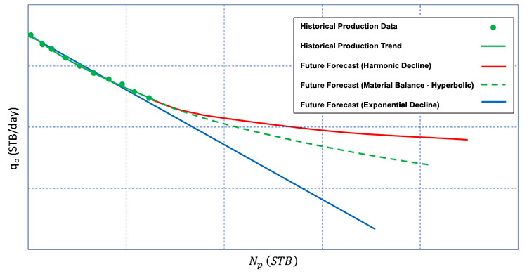
Using the relationships in Table 4.05, we can constrain (bracket) our production forecast from the Material Balance Method. This is shown in Figure 4.10. This figure illustrates why harmonic decline leads to an infinite EUR – the production can never achieve a zero rate and the area under the curve $(N_{p})$ becomes infinite.

Finally, the decline curves allow us to convert the $q_{o} - N_{p}$ forecasts to $q_{o} - t$ forecasts.

Graph showing historical trend with forecasts for Harmonic Decline, Material Balance, and Exponential Decline.

Figure 4.10: Comparison of Production Forecasts for the Material Balance and the Decline Curve Methods

Source: Greg King

Since decline curve analysis is a curve fitting, trend-line analysis technique, one important assumption in the use of decline curves is that whatever processes that occurred in the past that helped to establish the trend of the data must continue to occur into the future. This includes naturally occurring processes, such as, no changes in the reservoir drive mechanism, and operational changes, such as, no change to the specified flowing pressures of the wells, $p_{w f}$ .

[1] Arps, J. J.: “Analysis of Decline Curves,” SPE-945228-G, Trans. of the AIME (1945)

Navigation

EMS

Programs

Related Links