Lesson 4: Reservoir Engineering for Oil Reservoirs
4.0: Lesson Overview
Reservoir Engineering is the Petroleum Engineering Discipline which is concerned with the reservoir and oil accumulation oil as a whole. With the help of other petroleum professionals, such as drilling engineers, production engineers, and geologists, reservoir engineers attempt to optimize oil production from the reservoir or field in its entirety. Typical tasks performed by reservoir engineers working on oilfields include estimating the original oil-in-place, or STOOIP (Stock Tank Oil Originally In-Place), analyzing current production rate and pressure trends from the wells and the reservoir, forecasting future performance from these trends, and determining the Estimated Ultimate Recovery, or EUR, of a well, reservoir, or field.
There may be several methods available for performing the aforementioned tasks. Where multiple methods exist, we will discuss the more common methods available to the practicing reservoir engineer. In addition, we will discuss the assumptions inherent in each method.
Learning Objectives
By the end of this lesson, you should be able to:
- list some of the daily tasks performed by reservoir engineers;
- discuss two methods of calculating the Stock Tank Oil Originally in-Place, STOOIP, in an oil accumulation;
- calculate the STOOIP of a reservoir using the Volumetric Method and Material Balance Method;
- list and describe the five drive mechanisms associated with oil production given the proper data;
- list the major flow regimes experienced by vertical production wells;
- calculate the stabilized production rates from a production well given the current flow regime and given appropriate data;
- understand the concept of well damage or stimulation and know how to incorporate it into well production rate calculations;
- forecast future production from a reservoir or production well using the Material Balance Method and Decline Curve Analysis;
- list the three decline types considered by Arps Decline Curves;
- perform decline curve analysis using Arps Decline Curves; and
- understand the difference between economically recoverable oil and Estimated Ultimate Recovery (EUR).
Lesson 4 Checklist
| To Read | Read the Lesson 4 online material | Click the Introduction link below to continue reading the lesson 4 material |
|---|---|---|
| To Do | Lesson 4 Problem Set | Submit your solutions to the Lesson 4 Problem Set assignment in Canvas |
Please refer to the Calendar in Canvas for specific time frames and due dates.
Questions?
If you have questions, please feel free to post them to the Course Q&A Discussion Board in Canvas. While you are there, feel free to post your own responses if you, too, are able to help a classmate.
4.1: Introduction
In Lesson 3, we went over the basic rock, fluid, and rock-fluid interaction properties used by petroleum engineers on a daily basis. These form the building blocks for reservoir engineering calculations and forecasting procedures. In this lesson, we will discuss how these properties are used by reservoir engineers to predict how oil wells and oil fields behave.
For reservoir engineers, two main concerns are the estimation of the in-place fluids and the estimation of the rates and volumes of fluids produced from the production wells and from the field. For in-place fluid calculations, the Volumetric Method, which is based on static geological data, and the Material Balance Method, which is based on dynamic production and pressure data, are used. Both methods are commonly used in the oil and gas industry today.
For well performance, we will use Darcy’s Law in our analyses. In Lesson 3, we briefly discussed Darcy’s Law for fluid flow through porous media. The multi-phase version of Darcy’s Law (Equation 3.85), written for phase “ ” is:
Where is the pressure drop in the direction, which causes fluid flow. Darcy’s Law governs flow both at the well locations and in the interior of the reservoir. Consequently, this equation will be a fundamental tool for evaluating the performance of individual wells and the reservoir in its entirety.
Finally, we will discuss the application of material balance methods in the reservoir. Material balance is a tool used in many engineering disciplines; however, in this lesson, we will apply it to crude oil reservoirs. Put simply, material balance states that “matter can be neither created nor destroyed.” For our purposes, this implies that any change in mass in the reservoir must equal the mass being removed through the wells. As discussed earlier, material balance can be used for the estimation of the STOOIP (Stock Tank Oil Originally In-Place). In addition, it can be used for estimating the reservoir and field performance. We will discuss several material balance methods for crude oil reservoirs. In the next lesson, we will apply material balance to natural gas reservoirs.
4.2: Estimation of Stock Tank Oil Originally In-Place, STOOIP Using the Volumetric Method
As mentioned earlier, the Volumetric Method for STOOIP uses estimates of static geologic data to determine the volumes of the in-place fluids (crude oil, natural gas, and water). Static data are data which do not change with time due to oil and gas production. These static data are measured from core and log data.
For the volumetric method, the Gross Rock Volume (total rock volume of the reservoir zone of interest) and average values of porosity, fluid saturation, Net-to-Gross ratio (ratio of the volume of the productive reservoir to the total rock volume, i.e., the ratio of the volume of the reservoir that contributes to flow to the total rock volume), and the fluid formation volume factors ( ). While these properties can be determined on a point-by-point basis from core and log data at the well locations, development geologists use specialized geological modeling techniques to determine the inter-well properties and the averaged values of these properties.
By simply using the definition of reservoir volumes, the in-place volumes of the different reservoir fluids can be determined by:
Where:
- is the in-place volume of phase p, STB for crude oil and water or SCF for natural gas
- is the gross rock volume, ft3
- is the net-to-gross thickness ratio, fraction
- is the average net reservoir thickness, ft
- is the average gross reservoir thickness, ft
- is the average reservoir porosity, fraction
- is the average phase saturation, fraction
- is a unit conversion constant, 5.615 ft3/bbl for crude oil and water or 1.0 for natural gas
- is the average formation volume factor of phase , bbl/STB for crude oil and water or ft3/SCF for natural gas
In Equation 4.02, , is the average net thickness (the thickness of the reservoir that (1) contains hydrocarbons and (2) has sufficiently high permeability to contribute to flow), and is the average gross thickness (the total thickness of the reservoir). The net-to-gross ratio is simply the fraction that converts the total reservoir thickness to the thickness that contributes to hydrocarbon storage and flow in the reservoir. We can further define the gross rock volume as:
Where:
- is the gross rock volume, ft3
- 43,560 is a unit conversion constant, ft2/acre
- is the mapped area of the reservoir, acres
- is the average gross reservoir thickness, ft
Specifically, in standard SPE (Society of Petroleum Engineers) nomenclature, we have:
and
Where:
- 5.615 is a unit conversion constant, ft3/bbl
- is the Stock Tank Oil Originally In-Place (STOOIP), STB
- is the Original Gas In-Place (OGIP), SCF
- is the original water in-place, STB
Note that in Equation 4.04a, we used the saturation constraint, . To use the Volumetric Method to determine the Stock Tank Oil Originally In-Place, all of the pressure dependent properties are evaluated at the initial reservoir pressure, , as are all of the saturations, ,, and . All of the averages in these equations are averages over location (not averages over time).
The volumetric method for estimating the in-place volumes is considered to be less accurate than the material balance method. The reason for this is because of the use of all of the averages used in the volumetric method. This defect in the volumetric method can be improved by the use of an iso-contour parameter, . The iso-contour method calculates the composite property, , from the individual constituents:
The composite property, , is evaluated at the known at the points of Well Control (well locations where the properties , , , , and can be measured and are assumed to be known). Since the values that make up are all known at the points of well control, they can be used to evaluate without any averaging. Once values of are evaluated at the points of well control, they can then be averaged to determine . With the fluids in-place can be calculated with:
and
This approach reduces the averaging processes from the four averages required in Equation 4.04 to one required in Equation 4.06.
We will defer the discussion of the material balance method for the estimation of STOOIP until later in this lesson when we discuss field performance.
4.3: Drive Mechanisms in Oil Reservoirs
As with all gases and liquids in nature (weather fronts, sea and air currents, etc.), crude oil in the reservoir flows from locations of high pressure (the interior of the reservoir) to locations of low pressure (production wells). It is this pressure differential that is the driving force for fluid flow and production from wells. To start our discussion on fluid movement, we will begin with a discussion of the Drive Mechanisms in an oil reservoir. Drive mechanisms are the physical phenomena that occur in the reservoir that help to keep the reservoir pressures high.
There are five drive mechanisms that are associated with the Primary Production (production that occurs without any pressure maintenance supplied by fluid injection or by use of chemical, miscible, or thermal enhanced recovery methods) of a crude oil reservoir. These are:
Rock and fluid expansion occur due to the slightly compressible nature of crude oil, Interstitial (or Connate) Water, and reservoir rock. Interstitial, or connate, water is the initial water saturation in the reservoir at discovery. In Lesson 3, we saw that as pressure is reduced the compressibility of the rock and fluids (Equation 3.17, Equation 3.26, Equation 3.30, and Equation 3.43a) causes the volumes of the oil and water to expand and the pore-volume to shrink (equivalent to the rock grain volume expanding). All of these phenomena cause the pressure to remain higher than it would otherwise have been had they not been occurring (engineering analysis would indicate that if the fluids are expanding and the pore-volume is shrinking, then the in-situ fluids will be displaced to areas of low pressure).
We can think of rock and fluid expansion with the simple analogy of a water (or oil) filled balloon. If we fill the balloon with water, then the size of the balloon increases due to the increased pressure required to force the water into the balloon. In addition, if we pinch down on the balloon opening, then the water would remain in place inside of the balloon. In this example, the pore-volume in the reservoir is analogous to the water filled space in the balloon and the in-place fluid is the high-pressure water. Now, if we were to release the balloon opening to the low pressure atmosphere, then the pore-volume in the balloon would shrink and, to a lesser extent, the water inside the balloon would increase. These two effects cause the water to flow out of the balloon to the atmosphere. One conceptual issue with this analogy is the highly compressible nature of the rubber balloon. In a reservoir, the rock grains are many orders of magnitude less than the compressibility of rubber. Consequently, the flow of fluids from a hydrocarbon reservoir will not be as dramatic as that presented in this example.
Rock and fluid expansion occurs in most reservoirs; however, due to the small changes in volume associated with the slightly compressible nature of oil and water, and the low compressibilities associated with most reservoir rock, this drive mechanism has a very low recovery efficiency and typically accounts for less than five percent recovery of the STOOIP. In addition, in the presence of a free gas phase, its impact is dwarfed by the highly compressible nature of gas (note: gas expansion is excluded from rock and fluid expansion drive because the expansion of gas is included as separate drive mechanisms in solution gas drive and gas cap drive). Consequently, rock and fluid expansion may only be significant in undersaturated crude oil reservoirs (oil reservoirs discovered at pressures above the bubble-point pressure of the crude oil, .
Solution gas drive is caused by the solubility of natural gases in crude oils. This was discussed in Lesson 3 and is quantified with the oil property of the solution gas-oil ratio, . In undersaturated oil reservoirs, oil is found as a single-phase hydrocarbon fluid at discovery. As wells are drilled and put into production, the reservoir pressure declines (but supported by rock and fluid expansion) until it reaches the bubble-point pressure. At this time, gas comes out of solution and also begins to expand. It is the expansion of the gas that was originally in solution in the oil phase that we refer to as solution gas drive.
An analogy that we can use for solution gas drive is a bottle full of a carbonated beverage. If we were to shake a bottle of carbonated beverage with our thumb covering the bottle opening, the beverage would remain in the bottle. Now, if we were to remove our thumb from the bottle opening, then the gas in the beverage would come out of solution and expand in the bottle. This expansion of the liberated gas would drive both the beverage (and any gas remaining in solution in the beverage) and the free gas out of the bottle.
Typically, solution gas drive accounts for between 15 – 20 percent recovery of the STOOIP in normal oil reservoirs.
Gas cap drive is similar to solution gas drive; however, it only occurs in saturated oil reservoirs (oil reservoirs discovered below the bubble-point pressure of the crude oil). In saturated oil reservoirs, the free gas forms a Gas Cap (portion of the reservoir overlain by free gas due to gravity segregation). For example, the red colored region of the Numbi field in Figure 3.01 [1] is a gas cap. As wells are drilled and put into production, the pressure declines (again, other drive mechanisms may provide support to partially maintain the reservoir pressure), and the gas cap begins to expand. It is the expansion of the gas that was originally free in the reservoir that we refer to as gas cap drive.
Please note that during pressure decline, gas will also come out of solution. The expansion of this liberated gas is still referred to as solution gas drive. Thus, in this situation, we would have combined drives occurring simultaneously in the reservoir including gas cap drive and solution gas drive, and, to a lesser extent, rock and fluid expansion.
Gas cap drive can account for up to 30 percent recovery of the STOOIP depending on the size of the original gas cap.
Gravity drainage is another drive mechanism that can occur in both saturated and undersaturated oil reservoirs. In very thick reservoirs or in highly dipping reservoirs, gravity drainage can be a very effective drive mechanism and may account for up to 40 percent recovery of the STOOIP. In order to be effective, wells must be completed deep in the reservoir and must have a large Oil Column (reservoir depth containing oil) above the completion.
The last drive mechanism associated with oil reservoirs is aquifer drive, or water encroachment. If a reservoir is in contact with a water-bearing aquifer, then as the reservoir pressure declines, the rock and water in the aquifer expand and water is expelled from the aquifer and into the reservoir. This encroachment of water into the reservoir provides pressure support and helps to displace oil from the regions of the reservoir in contact with the aquifer to production wells. Aquifer drive may account for 35 – 45 percent recovery of the STOOIP depending on the size of the aquifer.
As previously discussed, these drive mechanisms commonly act simultaneously. When this occurs, we refer to the reservoir as a reservoir undergoing combined drive. Table 4.01 shows the drive mechanisms typically found in crude oil reservoirs and the maximum Recovery Factors (percentage of STOOIP recovered) typically observed in the field.
| Recovery Mechanism | Typical Recovery Efficiencies (Percent STOOIP) |
|---|---|
| Rock and Fluid Expansion | Up to 5 percent |
| Solution Gas Drive | 20 |
| Gas Cap Drive | 30 |
| Gravity Drainage | 40 |
| Aquifer Drive (Weak Aquifer) | 35 |
| Aquifer Drive (Strong Aquifer) | 45 |
| Combined Drive Mechanisms | 60 – very rarely this high |
The recovery factors shown in Table 4.01 may be a little deceptive since they represent the maximum recovery factors that can be expected from the reservoir for the different drive mechanisms. Typically, overall (combined) recovery factors from primary production rarely exceed 30 – 35 percent recovery of the STOOIP of the reservoir.
4.4: Performance of Oil Wells
4.4: Performance of Oil Wells section of this lesson will cover the following topics:
- 4.4.1: Stabilized Performance of Oil Wells [2]
- 4.4.1.1: Steady-State Flow of Oil to a Vertical Production Well with No Well Damage or Well Stimulation [3]
- 4.4.1.2: Steady-State Flow of Oil to a Vertical Production Well with Well Damage or Well Stimulation [4]
- 4.4.1.3: Steady-State Flow of Oil to a Vertical Production Well in Terms of the Average Pressure [5]
- 4.4.1.4: Pseudo Steady-State Flow of Oil to a Vertical Production well [6]
- 4.4.1.5: Inflow Performance Relationship for Stabilized Flow to an Oil Production Well [7]
- 4.4.2: Transient Performance of Oil Wells [8]
Note: You can access specific subsections of the lesson by clicking on the links above or continue reading through the lesson using the link below.
4.4.1: Stabilized Performance of Oil Wells
4.4.1: Stabilized Performance of Oil Wells section of this lesson will cover the following topics:
- 4.4.1.1: Steady-State Flow of Oil to a Vertical Production Well with No Well Damage or Well Stimulation [3]
- 4.4.1.2: Steady-State Flow of Oil to a Vertical Production Well with Well Damage or Well Stimulation [4]
- 4.4.1.3: Steady-State Flow of Oil to a Vertical Production Well in Terms of the Average Pressure [5]
- 4.4.1.4: Pseudo Steady-State Flow of Oil to a Vertical Production well [6]
- 4.4.1.5: Inflow Performance Relationship for Stabilized Flow to an Oil Production Well [7]
Note: You can access specific sections by clicking on the links above or continue reading through the lesson using the link below.
4.4.1.1: Steady-State Flow of Oil to a Vertical Production Well with No Well Damage or Well Stimulation
As stated earlier, the flow of oil to a production well is governed by Darcy’s Law. In this section, well damage is defined as a near-well permeability reduction (non-geological) caused by drilling or production. We will start our discussion by assuming that steady-state conditions prevail for the system. While steady-state conditions seldom occur in actual reservoirs, the analysis of production wells under these conditions forms the basis of the analysis methods of wells under more common reservoir conditions (pseudo steady-state conditions or transient, time-dependent conditions).
For steady-state analysis, we need to make the following assumptions:
- Flow is steady-state and Darcy’s Law applies and all of the inherent assumptions of Darcy’s Law are valid in the system.
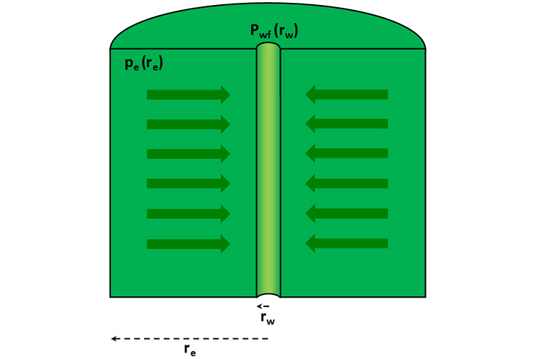
- The drainage volume is radial-cylindrical (see Figure 4.01).
- The drainage volume is bounded in the interior with a cylindrical well (radius equal to ) and kept at flowing well pressure of
- The drainage volume is bounded on the exterior with a cylindrical boundary (radius equal to ) which has an external pressure of ( < )
- The drainage volume is bounded on the top and bottom (constant height) no-flow boundaries.
- Within the drainage volume the rock properties are homogeneous (uniform with location).
- Within the drainage volume the rock properties are isotropic (uniform in all directions).
- Flow is horizontal.
With these assumptions, we can use the single-phase version of Darcy’s Law:
Now, for radial flow, we have:
Substituting into Darcy’s Law, we have:
The purpose of the negative sign in Equation 4.07 now becomes apparent: for a positive pressure gradient (pressure increasing with radius), flow is in the negative r-direction (flow is inward to the well: note direction of radii in Figure 4.01). Separating variables and integrating results in:
Now, using the assumption of a homogeneous permeability (constant with respect to location) and slightly compressible fluid (approximately constant , , and ), we have:
Performing the integration results in Equation 4.12 results in:
or,
Rearranging Equation 4.14 results in:
Equation 4.15 describes the steady-state flow of a single-phase, incompressible or slightly compressible fluid to a well in a radial-cylindrical drainage volume.
4.4.1.2: Steady-State Flow of Oil to a Vertical Production Well with Well Damage or Well Stimulation
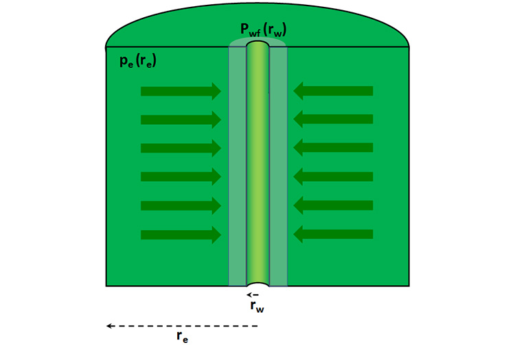
During drilling operations, filtrate from the drilling fluid can seep into the reservoir, causing several potential problems including swelling of clays, resulting in a restriction of pores causing a thin zone of absolute permeability degradation near the wellbore, and the formation of a two-phase zone, resulting in effective permeability impairment due to the impact of relative permeability near the well. In addition, fluid production may cause Fines Movement (movement of loose rock materials and debris) from the reservoir interior towards the well. Finally, the well may also be Stimulated (near well increase in permeability) by the use of a Hydraulic Fracturing Treatment or an Acid Stimulation Treatment.
This well damage or stimulation is introduced into the analyses with a Skin Factor (local, near-wellbore adjustment to the pressure drop – reduced or increased – due to permeability modification for reasons other than geological reasons). This damage or stimulation is called a “skin” factor because it results in a relatively small zone of increased pressure-drop (or increase) near the well. This skin zone is illustrated in Figure 4.02 as the light green zone adjacent to the well.
In reservoir Engineering, we quantify this additional pressure drop in the skin zone by use of a dimensionless parameter, . From Equation 4.14, we have:
By inspection, we can see that the left-hand side of this equation is dimensionless which implies that the right-hand side must also be dimensionless. Therefore, we can add our dimensionless skin factor, , to the left-hand side of the equation:
By doing this, in order to maintain the equality, we have either (1) modified the pressure drop, , if the production rate, , is fixed or, (2) modified the production rate if the pressure drop is fixed. Rearranging Equation 4.17 to the form of Equation 4.15 results in:
Well damage will occur if the permeability in the skin zone is less than the natural permeability of the reservoir, while stimulation will occur if the permeability in the skin zone is greater than the natural permeability of the reservoir. From Equation 4.18, we can see that if the skin factor, , is positive, then it results in a reduction in the production rate if the pressure drop is fixed. Therefore, a positive skin factor is an indication of damage to the well. On the other hand, a negative value of skin factor results in an increase in the production rate if the pressure drop is fixed. Therefore, a negative value of the skin factor is an indication of stimulation to the well.
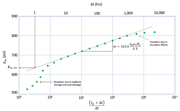
In the field, the skin factor can be determined from a pressure transient test, such as a pressure build-up test. In Lesson 3, we described a pressure build-up test and its analysis tool, the Horner Plot (see Figure 3.05). For convenience, this figure has been copied from Lesson 3 and is shown as Figure 4.03.
In that lesson, we discussed the Horner Plot in the context of field measurements of reservoir permeability. In that discussion, we saw that if we first produced a well at a stabilized rate, , for a certain period of time, , (the stabilized production time) and followed this by shutting in the well, then we could estimate the effective permeability to oil in the reservoir, , by the way that the shut-in pressures, , Built-Up (increased) over time. We quantified our analyses using the resulting Horner Plot:
Where:
Where:
- is the effective permeability to oil, md
- 162.6 is an equation constant
- is the oil production rate during the stabilized production period, STB/day
- is the oil viscosity, cp
- is the oil phase formation volume factor, bbl.STB
- is the slope of the Horner plot, in psi/cycle
- is the thickness of the reservoir, ft
- is the shut-in well pressure estimated from the linear portion of the plot, psi
Remember, as we discussed in Lesson 3, the effective permeability is the product of the relative permeability to oil and the absolute permeability of the rock formation:
We need to keep the relative permeability in our field calculations because all reservoirs will contain a water saturation (at the minimum it will be the irreducible water saturation, ). In addition to the effective permeability to oil, we can also determine the skin factor from the well test. For an arbitrary shut-in time increment, , the skin factor can be calculated from:
By convention, the time used in the skin analysis is normally taken to be one hour: . Substituting into Equation 4.22a:
Where:
- 1.1513 and 3.2275 are equation constants
- is the slope of the linear portion of the Horner plot, psi/cycle
- is the shut-in well pressure after 1 hr estimated from the linear portion of the Horner plot (see Figure 4.03), psi
- is the last measured flowing pressure during the stabilized production period ( at , i.e., ), psi
- is the total time duration of the stabilized production period, hrs
- is the time increment from the start of the well shut-in period, hrs
- is the effective permeability to oil, md
- is the porosity of the reservoir, fraction
- is oil viscosity, cp
- is total compressibility of the system, 1/psi
- is the well radius, ft
We can further simplify Equation 4.22b in cases where . In these cases, the expression in the first logarithmic term, , causing this term to vanish: remember, . In these cases, Equation 4.22b becomes:
When reservoir or production engineers design a pressure build-up test, they normally design it so that this approximation is valid. We can see from Equation 4.22, that in order to estimate the skin factor, we must first estimate the effective permeability, , and slope, , from Equation 4.19 and Equation 4.20.
You will notice that I use the term “estimate” when I discuss the application of these field methods for the determination of reservoir or well properties as opposed to “calculate”; this is intentional. While Equation 4.19 through Equation 4.22 are theoretically sound equations, (1) all of the properties used in them (, , , , , , , , , and ), to some degree have measurement error associated with them, and (2) many of the assumptions used in the equation development (uniform thickness, uniform permeability, etc.) may not be strictly applicable to our reservoir.
4.4.1.3: Steady-State Flow of Oil to a Vertical Production Well in Terms of the Average Pressure
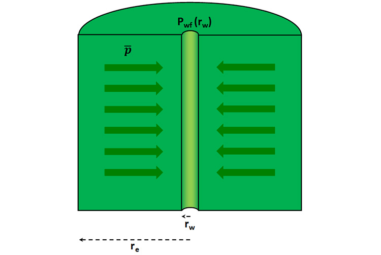
In our earlier discussions, we used the pressure drop from the external radius, at to determine the production rate, . In many situations, we may not know the reservoir pressure at ; however, we may know the average reservoir pressure, . In fact, as we will see during our discussion on material balance, this is actually the more common situation. This situation is depicted in Figure 4.04, where the pressure at the external radius, has been replaced with the average pressure, , in the interior of the drainage volume.
We can also develop equations for production rate for cases where we only know . To do this, we start with Equation 4.12. Rather than integrating this equation from to , we can change the limits of integration from to an arbitrary radius, , and the corresponding pressure at this radius, :
This results in an equation similar to Equation 4.14, but incorporating the arbitrary integration limits:
Solving for the pressure, , results in:
Equation 4.25 describes the Pressure Distribution (pressure as a function of location, which in our case is the pressure as a function radius) in the drainage volume. As one would expect, this equation indicates that as the radius, , increases away from the production well, the pressure also increases (i.e., fluids are flowing from regions of high pressure to the region of low pressure, the production well). The volumetric average of any property, (where upper case “” is any point-by-point property), can be calculated from:
Now, the volume of a cylinder is defined as:
Differentiating Equation 4.27 with respect to volume assuming a uniform thickness, , results in:
Substituting Equation 4.27 and Equation 4.28 into Equation 4.26 yields:
Now, substituting Equation 4.25 into Equation 4.29:
Performing the integration yields:
or,
or,
If we assume that , then . This is a very good assumption because the radius of the drainage volume of a well is typically on the order of hundreds or thousands of feet while the radius of the well is normally less than one foot. Using this approximation, Equation 4.31c becomes:
or, after rearranging:
Using the same methodology discussed earlier, we can also introduce the skin factor, , to account for well damage or stimulation:
Equation 4.34 is the relationship between the production rate of a liquid, , and the average reservoir pressure, . This equation has a similar form to that of Equation 4.19, but with two notable differences:
- The factor of ½ in the denominator of Equation 4.34
- The use of the average reservoir pressure in the drainage volume, , the pressure drop calculation in Equation 4.34
As I mentioned earlier, the use of, , has important consequences when applying material balance methods. We will discuss this later in this lesson.
4.4.1.4: Pseudo Steady-State Flow of Oil to a Vertical Production well
In all of our discussions on well performance, we assumed that Steady-State Conditions (time-invariant conditions) were occurring in the reservoir. Steady-state implies that nothing changes in the drainage volume with time or production. This simplification is not appropriate for most real production situations. Figure 4.05 shows the more common Transient Flow Conditions (time-dependent conditions) that occurs in the reservoir.
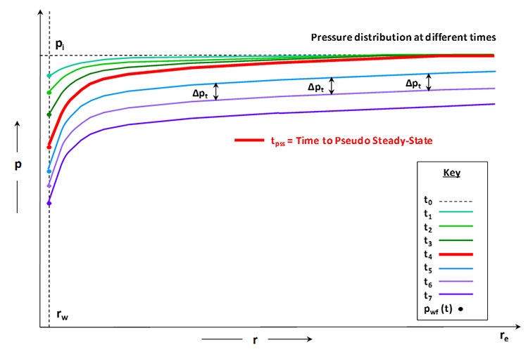
In this figure, the early-time pressures (green curves) form a pressure disturbance that over time propagates outward toward the external radius of the drainage volume, . At some point in time, this pressure disturbance reaches the external boundary (bold red curve). This time is referred to as the time to pseudo steady-state, . Pseudo steady-state is a flow regime which is defined by a uniform pressure drop from one time to the next, , that is equal everywhere in the drainage volume. This is illustrated in Figure 4.05 by the blue curves. The solid dual-headed arrows indicate that the pressure drop is the same at each radius in the reservoir.
The transient behavior of a radial-cylindrical drainage volume with uniform (constant) reservoir properties is governed by the partial differential equation (diffusivity equation):
I will derive this equation later in the lesson when we discuss fully transient flow; however, for the time being, we will consider its use in the context of pseudo steady-state flow. Without going into the details, the solution to this equation at times greater than can be approximated by:
Where:
- 5.615 is a unit conversion constant, ft3/bbl
- 1.127x10⁻³, 141.22, and 0.012648 are equation constants
- is the flowing well pressure, psi
- is the initial reservoir pressure, psi
- is viscosity, cp
- is the formation volume factor, bbl/STB
- is the liquid rate in STB/day
- is the permeability, md
- is the reservoir thickness, ft
- is the time, days
- is the porosity of the reservoir, fraction
- is total compressibility of the system, 1/psi
- is the external radius of the drainage volume, ft
- is the well radius, ft
Now, for slightly compressible liquids, we can calculate the average reservoir pressure by using the definition of compressibility:
In Equation 4.37, we set equal to the volume produced from the well over the time period , , and equal to the pore volume of the drainage volume in ft3. Substituting from Equation 4.37 into Equation 4.36 results in:
If we again assume that , then and the two time-dependent terms, , cancel. This results in:
Using the same methodology discussed earlier, we can also include the skin factor, , to account for well damage or stimulation:
We should not be surprised that the time dependent terms in Equation 4.38 canceled because during the pseudo steady-state flow regime, the pressure drop, , is uniform everywhere (see Figure 4.05). Thus, once the pressure distribution is formed at (red curve in Figure 4.05), the shape of the curve must remain intact throughout the remainder of the productive life of the well (assuming no changes in the production rate, ). The downward shift in the curves shown in Figure 4.05 are due to the reduction in the average reservoir pressure, , during pressure depletion.
4.4.1.5: Inflow Performance Relationship for Stabilized Flow to an Oil Production Well
The well performance equations that we have discussed to this point; Equation 4.18, Equation 4.34, and Equation 4.40; are known collectively as the well Inflow Performance Relationships, IPR (relationship between the flowing well pressure, , and the production rate, , from the well). Table 4.02 summarizes the flow regimes and the IPR equations.
| Steady-State Flow Regime | Pseudo Steady-State Flow Regime | |
|---|---|---|
| Pressure Distribution | ||
| In terms of at the external radius, , of the drainage volume | ||
| Drawdown | ||
| Productivity Index |
||
| IPR | ||
| In terms of in the interior of the drainage volume | ||
| Drawdown | ||
| Productivity Index |
||
| IPR | ||
| [A] Note, we did derive the equations in the shaded cells, but they are included for future reference. | ||
In Table 4.02, I introduced some new terminology. The pressure drop in these equations, , is referred to as the Drawdown or the Drawdown Pressure; while the term multiplying the drawdown is the referred to as Productivity Index, PI (sometimes the productivity index is also referred to by the symbol ). The oilfield units of the drawdown are psi; while the oilfield units of the productivity index are STB/(day psi).
Using this terminology, we can simplify the Inflow Performance Relationship to:
Where the appropriate definitions for the drawdown and productivity index are selected from Table 4.02 given the prevailing reservoir conditions (flow regime). Equation 4.41 is very useful for practical applications. In the field, we can change the well flowing pressure, , by changing the choke size on the well and measure the resulting stabilized production rate, . By doing this several times, we can estimate the productivity index from:
To do this, we must have some knowledge of the field pressure, typically measured by shutting in the well of interest or by shutting in Offset Wells (adjacent wells). Using this approach, the productivity of the well can be established without the need of knowing the individual well properties (, , , etc.) or the flow regime (steady-state or pseudo steady-state). The measured drawdowns and production rates provide the appropriate productivity index to allow for future well calculations.
In fact, we can use the field measured productivity indices even in cases with mixed flow boundaries/regimes. For example, we may have a situation where a strong aquifer is located south of a production well which keeps the southern external boundary of the drainage area nearly constant (steady-state). While north of this production well, pressure depletion may be occurring due to production from offset wells. In this situation, we do not need to make any assumptions regarding the flow regime, which best describes the well or what definitions of drawdown or productivity index we need to use. If we do the field measurement, then the test will provide the correct results for that specific well.
4.4.2: Transient Performance of Oil Wells
In our earlier discussions, we assumed that the well had produced for sufficient time to allow the pressures and production rates to stabilize. Transient Flow (time-dependent flow) describes the full time-dependence of these pressures and rates. If we were to produce a well at a constant rate, , then the flowing well pressure, , would behave as illustrated in Figure 4.06 on the following page.
4.4.2.1: Flow Regimes during Transient Flow
In Figure 4.06, the flowing well pressures, , are plotted as a function of time for a constant production rate. These flowing well pressures are the points, “•”, plotted in Figure 4.05. In this figure, several flow regimes are illustrated; some we have already discussed; others we have not.
For early times (solid red curve), the well pressure response is dominated well damage, well storage, or both. We have already discussed well damage earlier in this lesson. Well storage is the pressure response due to the liquids and gas in the well itself. Because the liquids are slightly compressible, and the gas is compressible, the flowing pressure of the well, , will be influenced by the compressibility of the fluids in the well.
The transient period (solid light green curve) in Figure 4.06 is flow regime that we are discussing in this subsection. The transient behavior of the well is described by the partial differential equation, Equation 4.30. The general solution to this equation forms the basis for Pressure Transient Analysis, PTA – such as the Pressure Build-Up Test and Horner Plot – that we discussed earlier.
The solid, dark green curve represents the late transient flow regime. As we have discussed, as a pressure disturbance caused by production travels through the reservoir, it will eventually encounter the boundaries of the drainage volume. For radial-cylindrical drainage areas in reservoirs with Homogeneous (uniform) and Isotropic (no directional preference) properties, this pressure disturbance comes into contact with all of the boundaries instantaneously (or at least over a short time interval).
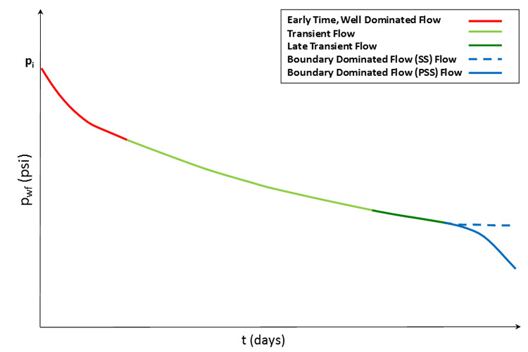
For square drainage areas, the pressure disturbance will contact the edges of the boundary first followed by the corners. For rectangular drainage areas, the pressure disturbance would first contact the boundaries on the short side of the rectangle, followed by the boundaries on the long side of the rectangle, and finally the corners of the rectangle. Therefore, for shapes other than cylindrical, the time duration for the pressure disturbance to contact all of the drainage volume boundaries may be drawn out. The late transient period is then defined as the period for the pressure disturbance to contact the first boundary through the last boundary of the drainage volume.
The boundary dominated period is shown by the two blue curves in Figure 4.06 with the dashed blue curve representing the steady-state flow regime and the solid blue curve representing the pseudo steady-state regime. We have already discussed these two flow regimes in detail in this lesson.
4.4.2.2: Derivation of the Diffusivity Equation in Radial-Cylindrical Coordinates
The derivation of the diffusivity equation in radial-cylindrical coordinates will be the last topic in our discussion on individual well performance. It also gives us the opportunity to introduce the topic of material balance, as we will use this concept in the following derivation.
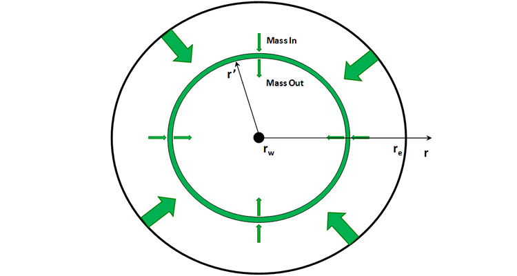
If we perform a mass balance on a thin ring or Representative Elemental Volume, REV, in the reservoir as shown in Figure 4.07, then we would have:
Equation 4.43 simply states that any mass entering the REV at its outer boundary less the mass exiting the REV at its inner boundary must be accumulating in the REV. We can elaborate on the definitions of terms in Equation 4.43 as:
and,
Where:
- 5.615 is a unit conversion constant, ft3/bbl
- is the liquid density, lb/ft3
- is the liquid rate, bbl/day
- is the radial coordinate in a radial-cylindrical coordinate system, ft
- is the radius of the representative elemental volume, REV, ft
- is time, days
- is the porosity of the reservoir, fraction
- REV is the bulk volume of the representative elemental volume, REV, ft3
- is the reservoir thickness, ft
Substituting Equation 4.44 through Equation 4.46 into Equation 4.43 results in:
or,
Dividing by the term results in:
Now, substituting Darcy’s Law, Equation 4.05 with and without the formation volume factor, B, (we want the flow rate in reservoir bbl/day not STB/day):
If we assume that the permeability, k, and the thickness, h, are uniform, then we have:
or,
or, after applying the chain rule:
Now, using the definition of compressibility for slightly compressible liquids:
Substituting Equation 4.51 into results Equation 4.50c in:
Equation 4.52 is the nonlinear diffusivity equation. We say that it is Nonlinear because the two density terms in the equation are functions of pressure. In this nonlinear form, we cannot solve the equation analytically (exactly). In order to obtain analytical solutions to this equation, we must first Linearize it. To do this, we apply the chain rule to the left-hand side of Equation 4.52:
or,
Note that the term, , is the first derivative squared and not the second derivative, . To complete the linearization process, we must assume the pressure gradient, , is small. If this is the case, then is very small, and we can remove it from Equation 4.53b:
or,
Which we can put into the compact format as:
or,
Where:
- 0.006328 is an equation constant (5.615 x 0.001127)
- is the radial coordinate in a radial-cylindrical coordinate system, ft
- is the pressure, psi
- is the porosity of the reservoir, fraction
- is the liquid viscosity, cp
- is the liquid compressibility, 1/psi
- is the reservoir permeability, md
- is time, days
- is the hydraulic diffusive , ft2/day
Equation 4.55 is the linear form of the diffusivity equation that describes the transient flow of a slightly compressible liquid through porous media. As we have already shown, solutions to this equation are useful in pressure transient analysis. The solutions to the diffusivity equation also have applications in the oil and gas production in:
- Rate Transient Analysis (analysis of time-dependent production rates)
- Type Curve Analysis (analysis of production rates using generalized, dimensionless plots)
- Unsteady-State Aquifer Performance (performance of aquifers in contact with hydrocarbon reservoirs)
The name Diffusivity Equation comes from the fact that this equation governs the diffusion process (with appropriate changes to the equation parameters and variables to make it relevant for diffusion). In addition, this equation also governs the process of heat conduction in solids, again, with appropriate changes to the equation parameters and variables.
4.5: Field Performance of Oil Reservoirs
To this point in the lesson, we have focused on the performance of individual wells. As reservoir engineers, we are also interested in the overall performance of the reservoir. It is important to note that we cannot simply sum the rates of the individual wells to determine the performance of the reservoir in its entirety. This is because Well Interference (interaction between wells) often occurs in the reservoir, which is not properly accounted for in our individual well analyses. This well interference occurs when the pressure disturbance caused by production from one well travels and comes into contact with the pressure disturbance caused by another well.
4.5: Field Performance of Oil Reservoirs section of this lesson will cover the following topics:
- 4.5.1: Field and Well Performance of Oil Reservoirs by Material Balance [11]
- 4.5.2: Field and Well Performance of Oil Reservoirs by Decline Curve Analysis [16]
Note: You can access specific subsections of the lesson by clicking on the links above or continue reading through the lesson using the link below.
4.5.1: Field and Well Performance of Oil Reservoirs by Material Balance
4.5.1: Field and Well Performance of Oil Reservoirs by Material Balance section of this lesson will cover the following topics:
- 4.5.1.1: Volumetric, Undersaturated Oil Reservoirs [12]
- 4.5.1.2: Non-Volumetric, Undersaturated Oil Reservoirs [15]
Note: You can access specific subsections of the lesson by clicking on the links above or continue reading through the lesson using the link below.
4.5.1.1: Volumetric, Undersaturated Oil Reservoirs
We were introduced to the concept of material balance earlier in this lesson when we discussed the derivation of the diffusivity equation. As we discussed in Lesson 2, an undersaturated oil reservoir is defined as a reservoir in which the initial pressure is greater that the bubble-point pressure of the crude oil. This results in a single, liquid hydrocarbon phase in the reservoir. As we discussed, there will be some water saturation in the reservoir also.
In this section, we will discuss the material balance method for Volumetric Reservoirs (reservoirs where the pore volume occupied by hydrocarbons remains constant with time – and pressure depletion). The Material Balance Method is applicable for both the reservoir in its entirety and to individual wells. From the volumetric method for estimating in-place fluids, we know that:
I have simplified this version of the equation (from Equation 4.04a) by assuming that the bulk volume in bbls, , is based on the net rock volume (that is, the net-to-gross ratio and the unit conversion constant, 5.615 ft3/bbl, have already been applied); the initial gas saturation is zero (because the reservoir is above the bubble-point pressure); and the water saturation is at its minimum value of .
In the Volumetric Method for STOOIP determination discussed earlier, all of the pressure dependent properties are evaluated at the initial reservoir pressure. Equation 4.56 is valid for any pressure conditions. If we evaluate Equation 4.56 twice, once at the initial conditions and once at some arbitrary, future condition (), then we would have:
and
Subtracting these two equations results:
Now, in this equation is the change in the oil-in-place (STB) in the reservoir from the initial condition to the future condition. Now, from material balance (mass is neither created nor destroyed), this change in mass is due to the expansion of the oil and must have been the mass of the oil produced from the wells during the time period, :
To make Equation 4.58b more convenient, we can substitute Equation 4.57a back into the equation:
or after multiplying both sides by the oil formation volume factor, , and rearranging:
Where:
- is the stock tank oil originally oil-in-place, STB
- is the oil-in-place at a future date, STB
- is the net rock volume, bbl
- is the porosity averaged over the reservoir, fraction
- is the irreducible water saturation averaged over the reservoir, fraction
- is the initial oil formation volume factor averaged over the reservoir, bbl/STB
- is the oil formation volume at a future time averaged over the reservoir, bbl/STB
- is the change in oil-in-place, STB
- is the oil production, STB
Equation 4.58d is the Material Balance Equation for volumetric reservoirs containing an undersaturated crude oil which remain above the bubble-point pressure. In this equation, the left-hand side represents the reservoir barrels removed from the reservoir through the production wells, while the right-hand side represents the expansion of oil in the reservoir. This equality is the general principle of material balance. We can use this equation in two ways:
- as a method to determine the STOOIP of the reservoir
- make future reservoir forecasts
4.5.1.1.1: Material Balance Method for Estimating the Stock Tank Oil Originally In-Place
In our earlier discussion on the estimation of Stock Tank Oil Originally In-Place, I mentioned that the two methods available for this task were the Volumetric Method and the Material Balance Method. We are now in a position to discuss the use of material balance for the estimation of the original oil-in-place in the reservoir. If we solve Equation 4.58d for STOOIP, , then we have:
Now in the field, if we accurately meter the oil production, , and actively measure average reservoir pressures (to evaluate ), then we can estimate and plot (on the y-axis) and on the x-axis (or, alternatively, time, t, on the x-axis). This results in a plot like that shown in Figure 4.08.
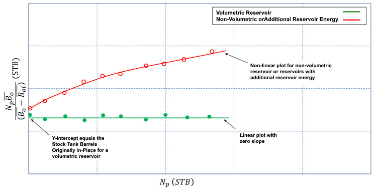
If all of the assumptions inherent in the development of Equation 4.59 are valid, then the data in Figure 4.08 should plot as a straight line with a zero slope and a y-intercept of (STOOIP), that is, the green curve in this figure. If these assumptions are not valid and there is more energy in the system other than the oil expansion, then the data will plot as a non-idealized curve, that is, the red curve.
The use of the material balance method to evaluate the original oil-in-place has several requirements associated with it. First, the Material Balance Method requires that production data are available. Therefore, it requires that the reservoir has been producing for some Historical Production Period (time period where the field has been on production). We must also have accurate estimates of the produced oil, , during this historical production period. This is typically a good assumption because we are selling the oil and must have accurate estimates for all of our sales obligations. In addition, it assumes that we have accurate estimates of the average reservoir pressure, , with time. This is part of a standard data acquisition program in the field and typically requires the involvement of reservoir engineers, production engineers, and geologists for good, representative estimates of average pressure. Finally, we must have accurate laboratory measurements of the formation volume factors, .
4.5.1.1.2: Material Balance Method for Making Future Reservoir Predictions
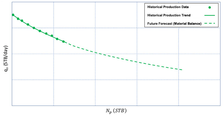
If we know the original oil-in-place from either the Volumetric Method or the Material Balance Method, then we can use Equation 4.58d to make future forecasts of reservoir performance with cumulative oil production, . We can do this by simply assuming average reservoir pressures, ; evaluating anticipated production at that pressure, , using Equation 4.58d; and estimating the stabilized oil production rate using either Equation 4.34 or Equation 4.40. Figure 4.09 shows a typical reservoir forecast in terms of .
In Figure 4.09, the historical production period is shown with the solid green data points and solid trendline, while the forecast is shown with the dashed green line. The noisy historical production data are a result of metering errors.
As I mentioned during our discussion on stabilized pressures, the use of in the drawdown calculation of the inflow performance is more consistent with material balance concept than the use of in the drawdown. This is because material balance is based on averaged reservoir properties. Therefore, for making predictions Equation 4.34 or Equation 4.40 should be used.
4.5.1.2: Non-Volumetric, Undersaturated Oil Reservoirs
In the development of Equation 4.58d, we assumed that the reservoir was volumetric (the pore-volume occupied by the oil was constant, and oil production was due to oil expansion only). If we remove this restriction and allow the pore-volume and rock to expand, then the volume of oil displaced to the wells (in bbl) becomes:
We have already seen that expansion of the original oil-in-place (in bbl) was described by Equation 4.58d:
The expansion of the water and rock can be determined by the definitions of compressibility. These definitions were given by Equation 3.21 and Equation 3.32. If we assume the initial pressure is the reference pressure, then:
Now, the expansion of water (in bbl) becomes:
Note that the use of this equation implies that the water volume is becoming larger (expanding) as the average pressure, decreases.
The change in pore-volume (in bbl) becomes:
Note that the use of this equation implies that the pore-volume is becoming smaller (contracting) as the average pressure, , decreases.
Both the increase in the water volume and the decrease in the pore-volume cause oil to be expelled from the reservoir, resulting in an increase in oil production (in bbl):
or,
Where:
- , , , and are the volume changes, bbl
- is the stock tank oil originally oil-in-place, STB
- is the initial oil formation volume factor averaged over the reservoir, bbl/STB
- is the oil formation volume at a future time averaged over the reservoir, bbl/STB
- is the net rock volume, bbl
- is the pore-volume, bbl
- is the pore-volume, bbl
- is the initial porosity averaged over the reservoir, fraction
- is the current porosity averaged over the reservoir, fraction
- is the irreducible water saturation averaged over the reservoir, fraction
- is the current water saturation averaged over the reservoir, fraction
- is the water compressibility, 1/psi
- is the rock, pore-volume compressibility, 1/psi
- is the current pressure averaged over the reservoir, psi
- is the current pressure averaged over the reservoir, psi
- is the oil production, STB
Equation 4.65b is the Material Balance Equation for Non-Volumetric, Undersaturated Reservoirs that remain above the bubble-point pressure. This equation will become more complicated as we add additional expansion terms. We can simplify the material balance equation using standard Society of Petroleum Engineering symbols as:
Where:
- is the sum of all Flow (production) from the reservoir, bbl
- is the stock tank oil originally oil-in-place, STB
- is the total Expansion of the system, bbl/STB
Again, we can use this equation for estimating the original oil-in-place and making future reservoir forecasts. To estimate the original oil-in-place, we divide Equation 4.66 by and plot (y-axis) versus (x-axis), (similar to how we generated Figure 4.08).
Equation 4.65b is valid for reservoirs with oil production caused by the expansion of the rock and fluids. It will now be instructive to go back to our discussion on the Drive Mechanisms for Oil Reservoirs. In that discussion, we listed all of the drive mechanisms associated with oil production and their approximate recovery factors (see Table 4.01). These drive mechanisms are:
- rock and fluid expansion
- solution gas drive
- gas cap drive
- gravity drainage
- natural aquifer drive (or water encroachment)
Without going into the details of the of each drive mechanism, Table 4.03 lists the expansion terms and production associated with each.
| Reservoir Drive Mechanisms in Terms of Standard Rock and Fluid Properties (from Lesson 3) | ||||
|---|---|---|---|---|
| Drive Mechanism | Expansion | Quantified | Production | Maximum Recoveries |
| Rock and Fluid Expansion | Oil Expansion | Up to 5 percent | ||
| Water Expansion (Interstitial Water) |
Up to 5 percent | |||
| Rock Expansion | Up to 5 percent | |||
| Solution Gas Drive | Solution Gas Expansion | 20 percent | ||
| Gas Cap Drive | Gas Cap Expansion | 30 percent | ||
| Gravity Drainage | Gravity Drainage | Not explicit in Material Balance Equation | 40 percent | |
| Natural Aquifer Drive | Water Encroachment | 45 percent | ||
| Production | ||||
| Drive Mechanism | Expansion | Quantified | Production | Maximum Recoveries |
| Production | Oil Production | |||
| Gas Production | ||||
| Water Production | ||||
Using the definitions shown in Table 4.03, we can rewrite Equation 4.66 as:
Where the entries in Equation 4.67 are listed in Table 4.04.
| Term | Description |
|---|---|
| Total volume of withdrawal (production) at reservoir conditions in bbl: and (SCF/STB) and (ft3/SCF) | |
| Cumulative oil Production in bbl | |
| Cumulative gas production in bbl | |
| Cumulative GOR (Gas-Oil Ratio) = Total gas produced over time divided by total oil produced over time. | |
| Cumulative water production in bbl | |
| Total expansion in the reservoir in bbl/STB: (bbl/STB) and (ft3/SCF). | |
| Total expansion of the oil and liberated gas dissolved in it. Expansion of the oil (above the bubble-point pressure) or shrinkage of the oil (below the bubble-point pressure due to liberation of gas) plus the expansion of the liberated gas | |
| is the ratio of gas cap volume, (SCF), to original oil volume, (bbl). A gas cap also implies that the initial pressure in the oil column must be equal to the bubble-point pressure. Note: is dimensionless. | |
| Expansion of the original of initial free gas (gas cap). | |
| Even though water has low compressibility, the volume of interstitial water in the system is normally large enough to be significant. The water will expand to fill the emptying pore-volume as the reservoir depletes. As the reservoir is produced, the pressure declines and the entire reservoir pore-volume is reduced due to compaction. The change in volume expels an equal volume of fluid (as production) and is additive in the expansion terms. | |
| If the reservoir is connected to an active aquifer, then once the pressure drop is communicated throughout the reservoir, the water will migrate into the reservoir resulting in a net water encroachment, in bbl. |
4.5.2: Field and Well Performance of Oil Reservoirs by Decline Curve Analysis
To this point in the lesson, everything that we have discussed is theoretical. That is, we developed these methods from first principles: Darcy’s Law, the definition of compressibility, basic rock and fluid properties, etc. Decline curve analysis is an Empirical Method (method based on observations) that is commonly used the oil and gas Industry. We will complete this lesson with a discussion on decline curves.
4.5.2: Field and Well Performance of Oil Reservoirs by Decline Curve Analysis section of this lesson will cover the following topics:
Note: You can access specific subsections of the lesson by clicking on the links above or continue reading through the lesson using the '>' link below.
4.5.2.1: Field and Well Performance with Arps Decline Curves
In a classic paper, J. J. Arps[1] took many observations from other investigators and concluded that the decline in the oil production rate, , over time from actual oil reservoirs could be described by the equations:
where the decline rate, , is a time dependent function:
Where:
- is the oil production rate, STB/day
- is the time, days (other units of time, such as months or years, can be used with an appropriate unit conversion constant)
- is the time dependent decline rate (time dependence defined by Equation 4.63), days-1
- is the initial decline rate (constant), days-1
- is a constant (typically used as a tuning parameter to match actual field data) and is in the range of , dimensionless
Decline curve analysis is essentially a curve fitting, or trend-line, analysis procedure where the form of the trend-line is developed from Arps[1] observations (Equation 4.68 and Equation 4.69). In this procedure, once the form of the trend-lines is established, we can use the parameters, , ,and to best match the data. We can develop these trend-lines or rate-time relationships if we integrate Equation 4.68 with respect to time. The resulting relationships have three forms depending on the value of the b-parameter.
[1] Arps, J. J.: “Analysis of Decline Curves,” SPE-945228-G, Trans. of the AIME (1945)
4.5.2.1.1: Exponential Decline (b=0)
If , then from Equation 4.69, , and we can integrate Equation 4.68 to obtain:
or,
Equation 4.70b is one of the rate-time relationships observed by Arps[1]. This equation is referred to as Exponential Decline because of the presence of the exponential term. We can also develop a rate cumulative production relationship by noting that:
Multiplying Equation 4.70b by and integrating results in:
or, after substituting Equation 4.70b into Equation 4.72a:
or, finally:
Equation 4.72 is the rate cumulative production relationship for exponential decline. The form of Equation 4.72b has two important applications. First, if we know the Abandonment Rate for the reservoir or well, , (rate at which the revenue from the oil sales would pay for the operating expenses of the reservoir or well), then we would have:
This would tell us the volume of oil that the reservoir or well would produce above the economic threshold. The second application of Equation 4.72b is if we would like to determine the production from the reservoir or well at an infinite time regardless of the economics. The volume of oil that can be recovered from a reservoir or well with no regard to the economics is called the Estimated Ultimate Recovery, or EUR, of the reservoir or well. We can determine the EUR by simply allowing the rate from reservoir or well to decline to 0 STB/day production rate (infinite time). That is:
The form of Equation 4.72c has one important application: to make future well forecasts. We can see that Equation 4.72c is a straight line in with a slope of (compare this straight-line relationship to the plot in Figure 4.09). Exponential decline is most often associated with the Rock and Fluid Expansion Drive Mechanism. In exponential decline, we have two parameters, and , with which to match the field data.
[1] Arps, J. J.: “Analysis of Decline Curves,” SPE-945228-G, Trans. of the AIME (1945)
4.5.2.1.2: Hyperbolic Decline (0<b<1)
If is in the range, , then the integration of Equation 4.68 and Equation 4.69 results in the rate-time relationship:
While a second integration with respect to time results in the rate-cumulative production relationship:
When the constant is in the range , we refer to the resulting production decline as Hyperbolic Decline. In hyperbolic decline, we have all three parameters, , , and , with which to match the field data.
4.5.2.1.3: Harmonic Decline (b=1)
If , then the integration of Equation 4.68 and Equation 4.69 results in the rate-time relationship:
While a second integration with respect to time results in the rate-cumulative production relationship:
When , we refer to the resulting production decline as Harmonic Decline. In harmonic decline, we have two parameters, and , with which to match the field data. Table 4.05 summarizes the results of Arps[1] Decline Curve Analyses.
| Relationship | Exponential Decline |
Hyperbolic Decline |
Harmonic Decline |
|---|---|---|---|
| Range of b-parameter | |||
| Rate-Time Relationship | |||
| Cumulative Production-Time Relationship | |||
| Rate-Cumulative Production Relationships | or |
or |
or |
| Maximum Economic Recovery | |||
| Estimated Ultimate Recovery, EUR |
Table 4.05 indicates that the EUR of a reservoir or well undergoing harmonic decline will be infinity. For this reason, a value of is considered to be an upper limit of this parameter. It is rarely used in any real analyses and is considered the theoretical maximum value of the parameter .
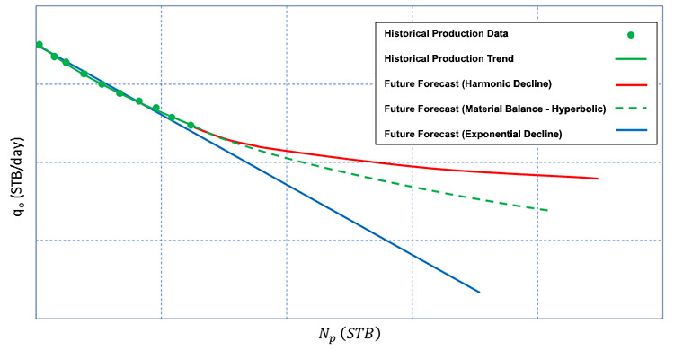
Using the relationships in Table 4.05, we can constrain (bracket) our production forecast from the Material Balance Method. This is shown in Figure 4.10. This figure illustrates why harmonic decline leads to an infinite EUR – the production can never achieve a zero rate and the area under the curve becomes infinite.
Finally, the decline curves allow us to convert the forecasts to forecasts.
Since decline curve analysis is a curve fitting, trend-line analysis technique, one important assumption in the use of decline curves is that whatever processes that occurred in the past that helped to establish the trend of the data must continue to occur into the future. This includes naturally occurring processes, such as, no changes in the reservoir drive mechanism, and operational changes, such as, no change to the specified flowing pressures of the wells, .
[1] Arps, J. J.: “Analysis of Decline Curves,” SPE-945228-G, Trans. of the AIME (1945)
4.6: Key Learnings
- Three of the key tasks performed by reservoir engineers are the estimation of the Stock Tank Oil Originally in-Place, STOOIP, in an oil reservoir or drainage volume, estimation of the stabilized production rate from a well, forecast future performance of an oil reservoir or well.
- Two common methods for calculating the STOOIP in an oil accumulation are:
- The Volumetric Method
- The Material Balance Method
- Drive mechanisms are the physical phenomena that keep reservoir pressures high and cause fluids to move to lower pressure areas in the reservoir. There are five drive mechanisms in an oil reservoir:
- Rock and fluid expansion
- Solution gas drive
- Gas cap drive
- Gravity drainage
- Natural aquifer drive (or water encroachment)
- The major flow regimes experienced by vertical production wells occur in sequence due to the pressure disturbance caused by production propagating radially outward from the well. These flow regimes are:
- Well dominated flow
- Transient flow
- Late transient flow
- Boundary dominated flow
- The stabilized production rates from a production well occur during the boundary dominate flow regime. These stabilized production rates are governed by the inflow performance relationships.
- Well damage or stimulation can occur in all production wells. Well damage/stimulation is quantified by the Skin Factor. A positive (+) skin factor results from well damage, while a negative (-) skin factor results from well stimulation.
- Two common methods for making future reservoir or well forecasts are:
- The Material Balance Method
- Decline curve analysis
- Exponential decline
- Hyperbolic decline
- Harmonic decline
4.7: Summary and Final Tasks
Summary
In this lesson, we discussed three very important tasks performed by reservoir engineers:
- estimation of the Stock Tank Oil Originally In-Place or STOOIP
- estimation of the stabilized production rate from a vertical oil well
- forecasting the future performance of oil reservoir and wells
We saw that there were two methods commonly used in the oil and gas industry estimating the STOOIP:
- the Volumetric Method
- the Material Balance Method
We discussed that of these two methods, the material balance method is typically assumed to be more accurate as it is based on dynamic data.
We also discussed the five Drive Mechanisms associated with oil reservoirs:
- Rock and fluid expansion
- Solution gas drive
- Gas cap drive
- Gravity drainage
- Natural aquifer drive (or water encroachment)
Later in the lesson, we saw how these drive mechanisms could be quantified and put into the material balance equation
We also discussed the stabilized production rates from vertical oil production wells. We saw that there were several flow regimes possible in a hydrocarbon reservoir that occurred at different stages in a well’s productive life. In Figure 4.06, we saw that these flow regimes occurred sequentially as the pressure disturbance caused by production propagates outward from the well. These flow regimes are:
- Well dominated flow
- Wellbore storage
- Damage/Stimulation
- Transient flow
- Late transient flow
- Boundary dominated flow
- Steady-state
- Pseudo steady-state
The well dominated flow regime is controlled by well properties and well damage/stimulation, not reservoir properties. The transient flow regime is governed by the diffusivity equation and is characterized by time-dependent rates and/or pressures. The onset of the late transient period occurs when the pressure disturbance from the production well reaches the first boundary of the drainage volume. The end of the late transient period occurs when the pressure disturbance reaches the last boundary of the drainage volume. The boundary dominated flow regime is the last regime experienced by the well. It is during this period that stabilized production occurs. Stabilized production is described by one of the Inflow Performance Relationships shown in Table 4.02.
For forecasting future reservoir or well performance, we discussed two methods:
- The Material Balance Approach
- Decline Curve Analysis
- Exponential decline
- Hyperbolic decline
- Harmonic decline
The Material Balance Method is an analytical (theoretically based) approach based on measured rock and fluid properties. It accounts for all drive mechanisms encountered in the field. Gravity drainage is considered implicitly in the choice of the datum depth used to evaluate the reservoir pressures. Decline curve analysis is an empirical (observation based) approach that uses trends in the observed data and analysis of these trends using simple mathematic expressions. Decline curve analysis is categorized based on the value of the b-parameter: exponential , hyperbolic , and harmonic .
Harmonic decline results in unrealistic EURs and is typically used as the theoretical limit for the b-parameter.
Final Tasks
Complete all of the Lesson 4 tasks!
You have reached the end of Lesson 4! Double-check the to-do list on the Lesson 4 Overview page [21] to make sure you have completed all of the activities listed there before you begin Lesson 5.