2.17 Learning Activity

This activity allows you to apply the concepts of time and space coordinates you learned in this lesson to a specific example of a solar energy conversion system. In the process, you will work with both Sun Chart and SAM software to model the performance of a PV array. You will be required to demonstrate your learned skills for Sun Chart interpretation, shadow tracking, and including shading information into SAM simulations.

PV Array System

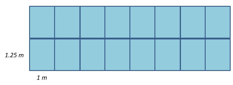
• A fixed-axis array of PV modules installed in the Baltimore MD area.
• The array consists of two rows of 8 modules stacked together (see more description and picture in Chapter 7 of the SECS Book), each module is 1.25 m in height and 1 m wide.

Figure 2.21: Sample array

Credit: Mark Fedkin © Penn State University is licensed under CC BY-NC-SA 4.0

• Orientation: azimuth -9^o (i.e. it is facing a few degrees East of South)
• Tilt: 35^o (fixed)
• The array is assumed to be part of a larger solar installation, meaning that a similar array positioned in the front can cast shadow to our array of interest.
• Spacing between the arrays in the field is 3 m.
• Nominal array capacity 4 kW
• Assume PV cells and modules are connected in series, so partial shading along the base will affect the entire array (simplified case).

Task

Model the effect of shading on the PV array performance (kWh of energy generated) over a year. So, in the end, you will need to produce the energy output data from the array for the full-sun and shaded scenarios and observe the difference.

Directions

1. SunChart. Create the Sun Chart for sun trajectory of the Baltimore, MD, location using the University of Oregon Solar Radiation Monitoring Laboratory solar tool. You are to use the polar sun chart in this activity. Download your Sun Chart diagram as a PDF file. You have seen examples of this in the videos included in this Lesson. You will use this chart further to put your shading information on.

2. Apply shading. Study the “Array Packing” example in Chapter 7 of the J. Brownson’s SECS Book, understanding how shading coordinates can be obtained for a specific system geometry. Plot all the critical points by shading coordinates given in Table 7.3 on your Sun Chart. Connect the points and show the shaded zone on your diagram (see lesson videos and textbook for more guidance on how to do it). You can use a graphics software for this purpose or do it by hand if that is easier.

   NOTE: the solar azimuth coordinates used by SunChart are different from those Brownson's book. The former considers 180^o as true south, while the latter considers 0^o as true south. So, you would need to convert the solar azimuths from the book by adding 180 in order to correctly plot the points on the SunChart.  

3. SAM Simulaton A (you have already downloaded SAM as instructed in Lesson 1):

   • Start a new PV project in SAM – choose Detailed PV Model - Residential Owner option when initiating a project
   • Under Location and Resource tab, input Baltimore, MD
   • Under System Design tab, input specifications for the system (4 kW nameplate capacity, array tilt and azimuth)
   • For the first round, do not include shading data
   • Run the simulation by pressing the blue 'Simulate' button at the bottom left of the screen
   • To get the monthly energy data in table, click on  DataTables tab on top. Then choose output variables: you need Monthly Energy (KWh) and total Annual Energy (kWh) for a single year. You can also find the latter by just summing up your monthly values.
   • Export your table to an Excel spreadsheet
4. Sam Simulation B. Repeat the same simulation as described in Step 3 now including the shading data. This is how: Save your project as a new file. Under 'Shading Layout' tab, click 'Edit Shading' button. Then, in the editing window, choose the option ‘Enable month by hour beam irradiance shading losses’. You will be given a table to input shading factors for each hour in each month. For simplicity, we will consider the same (averaged) shading factor for all days in the same month. Looking at your Sun Chart, input 0 for no shading, 100 for full shade, and 50 for borderline or changing conditions. Once done, run the SAM simulation and export data table as described in Step 3. (See demo video in Canvas for this step)

5. Discussion. Provide a brief discussion comparing your shaded and non-shaded results and what you learned from this activity. 

Submitting Your Work

Prepare a written report including the following results: 

• Sun Chart for Baltimore, MD with critical points and shaded zone plotted on it.
• Table of SAM simulation results for full sun and shaded scenarios. This table should contain monthly energy generated as well as total annual energy delivered by the array. In your energy performance table, your numbers should be rounded to the nearest whole kWh (no decimals).
• Screenshot of shading factor table from SAM.
• A paragraph with a discussion of your results.

Upload your report file to the Lesson 2 Learning Activity DropBox in PDF or docx format.

Grading Criteria

• Sun Charts (10 pt). This part will be graded based on your ability to plot the calculated critical points and identify shaded versus non-shaded conditions for the system at the specific time and location.
• Energy Tables (10 pt). You will be given 1 pt per month based on the reasonable correctness of the numerical values. The purpose is not necessarily to get the exact "right" answer, but rather to have done the process and understand what you are doing. So discrepancies within +/- 30 kWh will not cause point deductions.
• Discussion (5pt).
• Screenshot of the Table with shading factors used for SAM simulation (5 pt). 

Deadline

See the Canvas Calendar for specific due dates.