7.2 Electromagnetic Radiation

Most remote sensing instruments measure the same thing: electromagnetic radiation. Electromagnetic radiation is a form of energy emitted by all matter above absolute zero temperature (0 Kelvin or -273° Celsius). X-rays, ultraviolet rays, visible light, infrared light, heat, microwaves, and radio and television waves are all examples of electromagnetic energy.

Figure 7.3. The Electromagnetic Spectrum showing segments of the spectrum with associated wavelengths(nm). Also, note the emittance curves for the Sun and Earth provided in the graph. Use this link to access a larger version of the image.

Electromagnetic Wave Spectrum by Horst Frank is licensed CC-BY-SA 4.0 International

The graph above shows the relative amounts of electromagnetic energy emitted by the Sun and the Earth across the range of wavelengths called the electromagnetic spectrum. Values along the horizontal axis of the graph range from very long wavelengths (TV and radio waves) to very short wavelengths (cosmic rays). Hotter objects, such as the sun, radiate energy at shorter wavelengths. This is exemplified by the emittance curves for the Sun and Earth, depicted in Figure 7.3. The sun peaks in the visible wavelengths, those that the human eye can see, while the longer wavelengths that the Earth emits are not visible to the naked eye. By sensing those wavelengths outside of the visible spectrum, remote sensing makes it possible for us to visualize patterns that we would not be able to see with only the visible region of the spectrum.

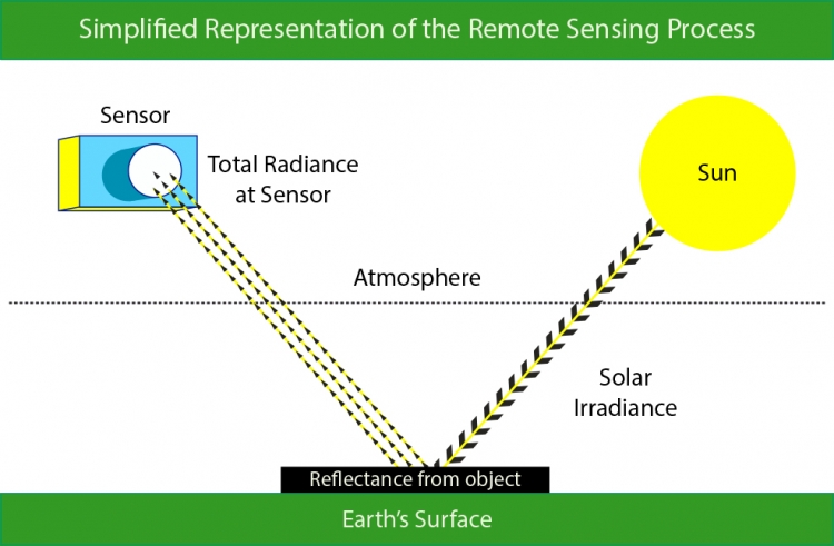
The remote sensing process is illustrated in Figure 7.4. During optical remote sensing, a satellite receives electromagnetic energy that has been (1) emitted from the Sun, and (2) reflected from the Earth’s surface. This information is then (3) transmitted to a receiving station in the form of data that are processed into an image. This process of measuring electromagnetic energy is complicated by the Earth’s atmosphere. The Earth's land surface reflects about three percent of all incoming solar radiation back to space. The rest is either reflected by the atmosphere, or absorbed and re-radiated as infrared energy. As energy passes through the atmosphere, it is scattered and absorbed by particles and gases. The absorption of electromagnetic energy is tied to specific regions in the electromagnetic spectrum. Areas of the spectrum which are not strongly influenced by absorption are called atmospheric windows. These atmospheric windows, seen above in Figure 7.3, govern what areas of the electromagnetic spectrum are useful for remote sensing purposes. The ability of a wavelength to pass through these atmospheric windows is termed transmissivity. In the following section, we will discuss how the energy we are able to sense can be used to differentiate between objects.

Figure 7.4. The generalized remote sensing process. Solar irradiance is emitted from the Sun, travels through the Earth's atmosphere and then reflects off objects on the Earth's surface. Some of the energy is captured by the sensor.

Dutton Institute, Penn State

7.2.1 Visual Interpretation Elements

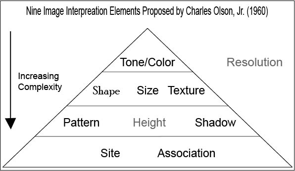
You have seen how a sensor captures information about the reflectance of electromagnetic energy. But, what can we do with that information once it has been collected? The possibilities are numerous. One simple thing that we can do with a satellite image is to interpret it visually. This method of analysis has its roots in the early air photo era and is still useful today for interpreting imagery. The visual interpretation of satellite images is based on the use of image interpretation elements, a set of nine visual cues that a person can use to infer relationships between objects and processes in the image.

Figure 7.5. Representation of Nine Image Interpretation Elements Proposed by Charles Olson, Jr. (1960)

Credit: (adapted from Estes 1983).

7.2.1.1 Size

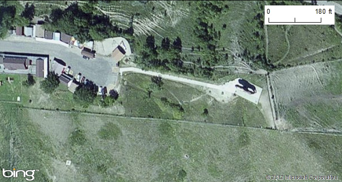
The size of an object in an image can be visually discerned by comparing the object to other objects in the scene that you know the size of. For example, we know the relative size of a two-lane highway, but we may not be familiar with a building next to it. We can use the relative size of the highway and the building to judge the building’s size and then (having a size estimate) use other visual characteristics to determine what type of building it may be. An example of the use of size to discern between two objects is provided in figure 7.6.

Figure 7.6. In this image we can see a buffalo, however, when we compare its size to the nearby buildings we are quick to notice that it cannot be a living buffalo because it is much bigger than any of those buildings. In fact, this buffalo monument is located in Jamestown, North Dakota.

Credit: Bing Maps.

7.2.1.2 Shape

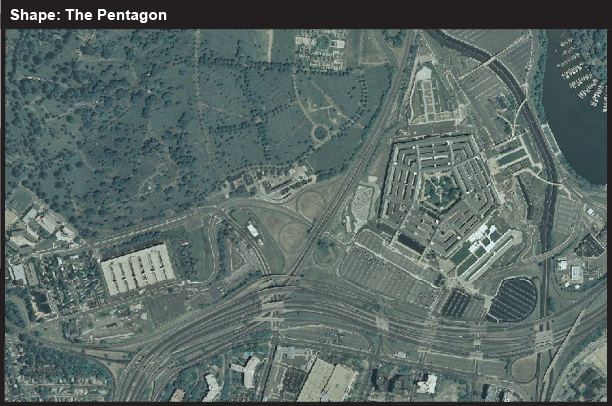
There are not many cases where an individual object has a distinct shape, and the shape of an object must be considered within the context of the image scene. There are several examples where the shape of an object does give it away. A classic example of shape being used to identify a building is the Pentagon, the five-sided building in figure 7.7 below.

Figure 7.7. The Pentagon is easily identified in this urban scene because of its unique shape.

Credit: Bing Maps.

7.2.1.3 Tone/Color

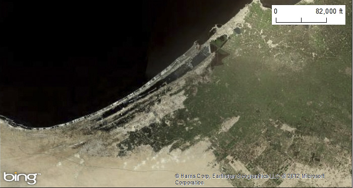
In grayscale images, tone refers to the change in brightness across the image. Similarly, tone refers to the change in color in a color image. Later in this chapter, we will look at how we can exploit these differences to automatically derive information about the image scene. In Figure 7.8 below, you can see that the change in tone for an image can help you discern between water features and forests.

Figure 7.8. Using color to discern between bodies of water (dark blue), desert, and a green vegetation.

Credit: Bing Maps.

7.2.1.4 Pattern

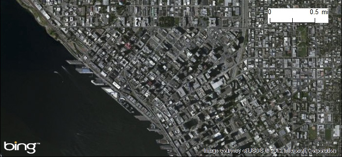
Pattern is the spatial arrangement of objects in an image. If you have ever seen the square plots of land as you flew over the Midwest, or even in an aerial image, you have probably used the repetitive pattern of those fields to help you determine that the plots of land are agricultural fields. Similarly, the patten of buildings in a city allows you to recognize street grids as in Figure 7.9 below.

Figure 7.9. The repetition of the buildings in Seattle provide a pattern which makes it easier to identify roadways in this image.

Credit: Bing Maps.

7.2.1.5 Shadow

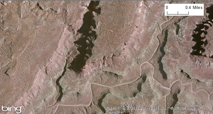
The presence or absence of shadows can provide information about the presence or absence of objects in the image scene. In addition, shadows can be used to determine the height of objects in the image. Shadows also can be a hindrance to image interpretation by hiding image details, as in Figure 7.10 below.

Figure 7.10. Shadow can be used to discern between the different heights of plateaus in this image of the Grand Canyon. We see dark shadows for tall straight relief and soft gray shadows along river dendrites.

Credit: Bing Maps.

7.2.1.6 Texture

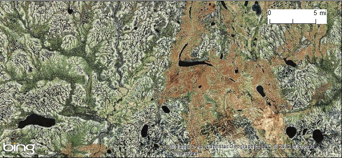
The term texture refers to the perceived roughness or smoothness of a surface. The visual perception of texture is determined by the change in tone, for example, a forest is typically very rough looking and contains a wide range of tonal values. In comparison, a lake where there is little to no wind looks very smooth because of a lack of texture. Whip up the winds though, and the texture of that same body of water soon looks much rougher, as we can see in Figure 7.11.

Figure 7.11. The texture in this figure, along with color, leads one to see that the image is of a tundra environment. The smooth dark ponds contrast with the rough frozen texture of the land.

Credit: Bing Maps.

7.2.1.7 Association

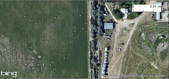
Association refers to the relationships that we expect between objects in a scene. For example, in an image over a barnyard you might expect a barn, a silo, and even fences. Also, the placement of a farm is typically in rather rural areas. You would not expect a dairy farm in downtown Los Angeles. Figure 7.12 shows an instance where association can be used to identify a city park.

Figure 7.12. In this scene of a farm in Wyoming, we can see many little white blocks in the pasture. These white blocks can be identified as hay bales by their presence near the barns. In another image, such as an urban scene, a similar white block may be tables or other objects related to an urban environment.

Credit: Bing Maps.

7.2.1.8 Site

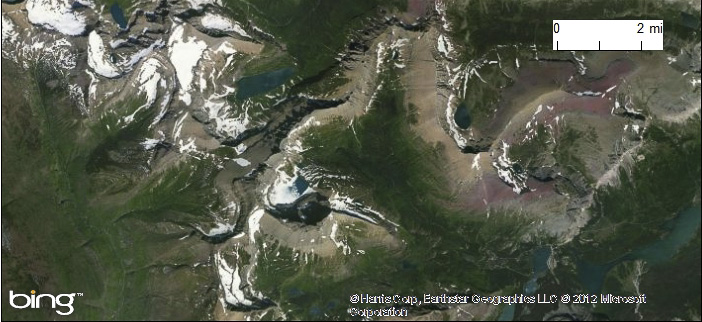
Site refers to topographic or geographic location. The context around the feature under investigation can help with its identification. For example, a large sunken hole in Florida can be easily identified as a sink hole due to limestone dissolution. Similar shapes in the desserts of Arizona however are more likely to be impact craters resulting from meteorites.

Figure 7.13. This image shows Grinell Glacier. By noting the fact that it is in Glacier National Park, that you can see crevasses, and that it is on the side of a mountain, we are able to determine that the snow is actually a glacier and not just normal snowfall.

Credit: Bing Maps.

7.2.2 Spectral Response Patterns

You have now seen the possibility of visually interpreting an image. Next, you will learn more about how to use the reflectance values that sensors gather to further analyze images. The various objects that make up the surface absorb and reflect different amounts of energy at different wavelengths. The magnitude of energy that an object reflects or emits across a range of wavelengths is called its spectral response pattern.

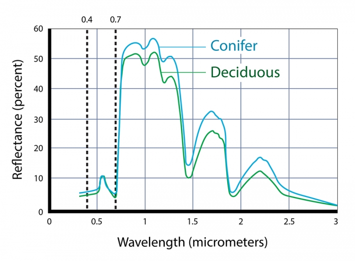
The following graph illustrates the spectral response pattern of coniferous and deciduous trees. The chlorophyll in green vegetation absorbs visible energy (particularly in the blue and red wavelengths) for use during photosynthesis. About half of the incoming near-infrared radiation is reflected (a characteristic of healthy, hydrated vegetation). We can identify several key points in the spectral response curve that can be used to evaluate the vegetation.

Notice that the reflectance patterns within the visual band are nearly identical. At longer, near- and mid-infrared wavelengths, however, the two types are much easier to differentiate. As you'll see later, land use and land cover mapping were previously accomplished by visual inspection of photographic imagery. Multispectral data and digital image processing make it possible to partially automate land cover mapping, which, in turn, makes it cost effective to identify some land use and land cover categories automatically, all of which makes it possible to map larger land areas more frequently.

Figure 7.14. This spectral response pattern of a conifer forest and a deciduous forest illustrates the places along the electromagnetic curve where we can differentiate between the two forest types.

Dutton Institute, Penn State

Spectral response patterns are sometimes called spectral signatures. This term is misleading, however, because the reflectance of an entity varies with its condition, the time of year, and even the time of day. Instead of thin lines, the spectral responses of water, soil, grass, and trees might better be depicted as wide swaths to account for these variations.

7.2.2.1 Spectral Indices

One advantage of multispectral data is the ability to derive new data by calculating differences, ratios, or other quantities from reflectance values in two or more wavelength bands. For instance, detecting stressed vegetation amongst healthy vegetation may be difficult in any one band, particularly if differences in terrain elevation or slope cause some parts of a scene to be illuminated differently than others. However, using the ratio of reflectance values in the visible red band and the near-infrared band compensates for variations in scene illumination. Since the ratio of the two reflectance values is considerably lower for stressed vegetation regardless of illumination conditions, detection is easier and more reliable.

7.2.2.2 Normalized Vegetation Index

Besides simple ratios, remote sensing scientists have derived other mathematical formulae for deriving useful new data from multispectral imagery. One of the most widely used examples is the Normalized Difference Vegetation Index (NDVI). NDVI can be calculated for any sensor that contains both a red and infrared band; NDVI scores are calculated pixel-by-pixel using the following algorithm:

NDVI = (NIR - R) / (NIR + R)

R stands for the visible red band, while NIR represents the near-infrared band. The chlorophyll in green plants strongly absorbs radiation within visible red band during photosynthesis. In contrast, leaf structures cause plants to strongly reflect radiation in the near-infrared band. NDVI scores range from -1.0 to 1.0. A pixel associated with low reflectance values in the visible band and high reflectance in the near-infrared band would produce an NDVI score near 1.0, indicating the presence of healthy vegetation. Conversely, the NDVI scores of pixels associated with high reflectance in the visible band and low reflectance in the near-infrared band approach -1.0, indicating clouds, snow, or water. NDVI scores near 0 indicate rock and non-vegetated soil.

The NDVI provides useful information relevant to questions and decisions at geographical scales ranging from local to global. At the local scale, the Mondavi Vineyards in Napa Valley California can attest to the utility of NDVI data in monitoring plant health. In 1993, the vineyards suffered an infestation of phylloxera, a species of plant louse that attacks roots and is impervious to pesticides. The pest could only be overcome by removing infested vines and replacing them with more resistant root stock. The vineyard commissioned a consulting firm to acquire high-resolution (2-3 meter) visible and near-infrared imagery during consecutive growing seasons using an airborne sensor. Once the data from the two seasons were georegistered, comparison of NDVI scores revealed areas in which vine canopy density had declined. NDVI change detection proved to be such a fruitful approach that the vineyards adopted it for routine use as part of their overall precision farming strategy (Colucci, 1998).