
Absolute Versus Relative Sea Level Change
In fact, changes in the height of the ocean as a result of melting ice or warming seas (absolute or eustatic sea level change) only tell part of the story. The level of the ocean can also change because the underlying land is rising or falling with respect to the ocean surface. Such relative sea level change usually affects a local or regional area, and in numerous cases, is actually outpacing the rate of sea level change.
Relative sea level changes can be caused by plate tectonic forces. For example, the Great Japan earthquake on March 11, 2011, caused part of the island of Honshu to rise up by nearly three meters. The sea floor can also drop when huge amounts of sediment are deposited by rivers and deltas. The weight of the sediment depresses the underlying crust, often at a faster rate than the sediment is being deposited. This process is happening along the east coast of the US today in places along the coasts of Maryland, North Carolina and Georgia, and the Gulf Coast, especially in the Mississippi Delta region. In parts of Florida where large amounts of water have been pumped out of aquifers for water supply, the land is also subsiding rapidly.
Relative
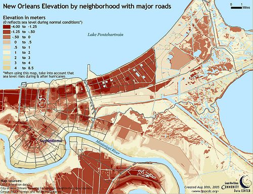
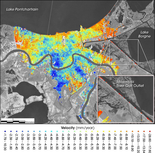
One of the most drastic examples of relative sea level change is around New Orleans, where sea level is rising with respect to the land at alarming rates. The map below left shows that in parts of the city, the land surface is subsiding at nearly 3 cm per year! There are two additional alarming parts of this story. The first is that the rates actually may have been faster in the past and have the potential to increase again; the second is that parts of the city already lie 4 meters below sea level (see map below left). The causes of the New Orleans subsidence are partially natural. The city sits on delta sediments that are accumulating very rapidly and causing the underlying crust to subside due to their weight. However, humans are also responsible. Draining wetlands, over pumping aquifers and diverting floodwaters from the Mississippi River are all contributing to rapid subsidence.
The New Orleans subsidence map is an excellent example of relative sea level change. However, the fact that the land the city is built upon is subsiding so rapidly makes it more prone than most areas to absolute sea level rise as a result of warming oceans and melting ice sheet. Late in this module, we will observe some of the changes the city has made to combat both sources of sea level rise. However, the rates of subsidence are so rapid that some scientists are advising retreat from the coast as the wisest option from an economic and safety point of view.
New Orleans Flooding Maps
Changing sea levels around New Orleans and other regions are at least partially part of natural changes that have been occurring for hundreds of millions of years; absolute and relative sea level has been rising and falling continuously through geologic time. As the coastline has moved landward with sea level rise (a change called transgression), thick marine deposits are laid down, beach sands over coastal marsh sediments, deeper shelf deposits over beach sands, and slope sediments over shelf deposits. The marine deposition is generally considered to be continuous. Conversely, as the coastline has moved back seaward (a change called regression), shelf deposits are superimposed on slope deposits and marsh deposits are laid down over beach sands. Rock sequences on land show these characteristic sequences, for example, coals deposited in swamps, overlain by beach and shelf sands.
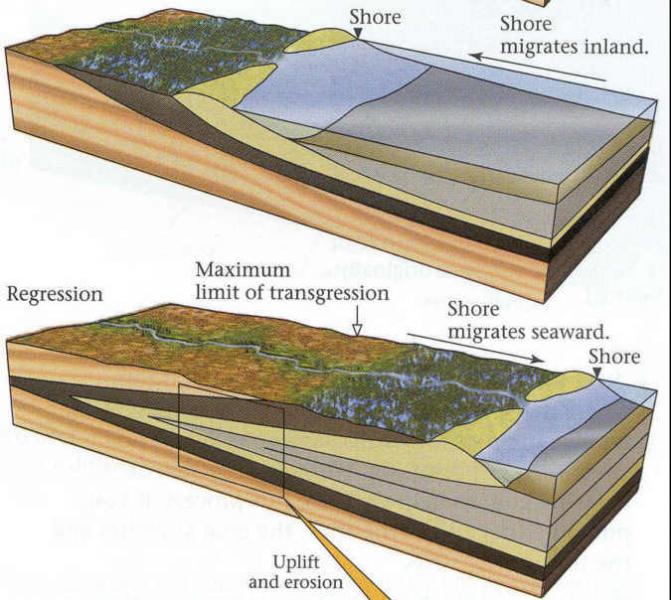
The diagrams illustrating coastal changes due to sea level fluctuations. The top diagram shows a transgression phase where the shore migrates inland, with the shoreline moving over land due to rising sea levels, depicted with a blue ocean layer encroaching onto a green and brown landscape. The bottom diagram illustrates a regression phase, labeled "maximum limit of transgression," where the shore migrates seaward due to falling sea levels, exposing more land. It highlights uplift and erosion with a yellow arrow, showing sediment layers and a river system forming as the ocean (blue) retreats from the land (green and brown).
- Diagram Overview
- Type: Two cross-sectional views of coastal changes
- Top Diagram (Transgression)
- Description: Shore migrates inland
- Visual: Blue ocean layer encroaching on green and brown land
- Label: Shore migration inland
- Bottom Diagram (Regression)
- Description: Shore migrates seaward
- Labels: Maximum limit of transgression, shore migration seaward
- Visual: Blue ocean retreating, exposing green and brown land
- Additional Process: Uplift and erosion
- Visual: Yellow arrow indicating uplift and sediment layers
- Features: River system forming on exposed land
Once this regression reaches a certain point, much of the shelf becomes subaerial and characterized by sporadic deposition and erosion. This erosion makes a surface that is called an unconformity, which is essentially a gap in time. The unconformities end up bounding a package of strata that is deposited by one individual sea level rise and fall. Such packages are known as sequences. The multiple sea level rises and falls have produced sequence upon sequence underneath the continental shelf and slope. These sequences hold within them the history of relative and absolute sea level change.
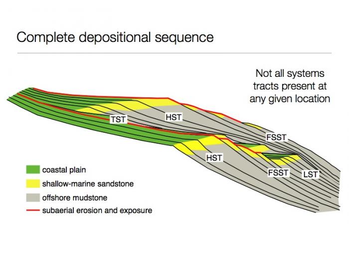
The diagram Illustrates a cross-sectional view of layered sediment deposits. It shows various systems tracts labeled TST, HST, FSST, and LST, representing different phases of sediment deposition. The layers are color-coded: green for coastal plain, yellow for shallow-marine sandstone, and gray for offshore mudstone with subaerial erosion and exposure. A note indicates that not all systems tracts are present at any given location. Red lines mark the boundaries between the tracts.
- Diagram Overview
- Title: Complete depositional sequence
- Type: Cross-sectional view of sediment layers
- Systems Tracts
- TST (Transgressive Systems Tract)
- HST (Highstand Systems Tract)
- FSST (Falling Stage Systems Tract)
- LST (Lowstand Systems Tract)
- Visual: Labeled with red boundary lines
- Layer Types
- Coastal Plain
- Color: Green
- Shallow-Marine Sandstone
- Color: Yellow
- Offshore Mudstone and Subaerial Erosion and Exposure
- Color: Gray
- Coastal Plain
- Additional Note
- Text: Not all systems tracts present at any given location
Geophysicists can image the subsurface using a technique called reflection seismology. Basically, elastic waves from ships are produced by airguns, these waves travel down through the ocean and reflect back off the seafloor and the layers underneath it. It turns out that the unconformities between the sequences reflect a lot more energy than the conformable layers within the sequences, so the sequences can be mapped precisely using reflection seismology. Individual sequences can be age dated using microfossils (see Module 1) and in this way, the history of sea level can be determined. This technique is known as sequence stratigraphy.
Absolute
So, the big question is how we know whether sequence stratigraphy reflects relative sea-level change caused by changes in subsidence, sedimentation, and sediment loading, as we discussed in the previous section, or absolute or eustatic sea level changes? The way individual sequences can be confirmed as eustatic is when they are observed on different continental margins (it would be difficult to imagine how regional subsidence, sedimentation patterns, and sediment loading would impact margins in a different part of the world at the same time).
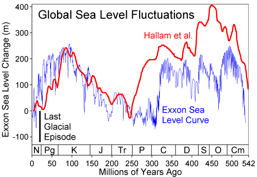
The graph shows sea level changes in meters on the y-axis (-150 to 400 m) over millions of years ago on the x-axis (0 to 542 million years). The graph features two data sets: a red line labeled "Hallam et al." and a blue line labeled "Exxon Sea Level Curve." Both lines fluctuate significantly, indicating sea level rises and falls across geological periods marked on the x-axis: Neogene (N), Paleogene (Pg), Cretaceous (K), Jurassic (J), Triassic (Tr), Permian (P), Carboniferous (C), Devonian (D), Silurian (S), Ordovician (O), and Cambrian (Cm). A notable drop occurs during the Last Glacial period, around 0-50 million years ago, with sea levels falling to around -100 m.
- Graph Overview
- Title: Global Sea Level Fluctuations
- Type: Line graph
- Time Period: 0 to 542 million years ago
- Axes
- Y-axis: Sea level change (-150 to 400 m)
- X-axis: Millions of years ago (0 to 542)
- Data Sets
- Hallam et al.: Red line
- Exxon Sea Level Curve: Blue line
- Geological Periods
- Neogene (N), Paleogene (Pg), Cretaceous (K), Jurassic (J), Triassic (Tr), Permian (P), Carboniferous (C), Devonian (D), Silurian (S), Ordovician (O), Cambrian (Cm)
- Key Event
- Last Glacial: Around 0-50 million years ago
- Sea Level: Drops to around -100 m
- Last Glacial: Around 0-50 million years ago
- Trend
- Description: Both lines show significant fluctuations, with peaks and troughs across periods
As it turns out, sea level curves such as the ExxonMobil curve have a hierarchy of cycles. Very short frequency cycles with frequencies lasting a few thousand years are superimposed on cycles with millions of year frequencies, and these are superimposed on long frequency cycles lasting 100s of millions of years. The current chart has five orders of cycles, all superimposed. The longer order cycles are almost certainly eustatic in origin. The shorter order cycles which cannot unequivocally be matched between continents are likely relative sea level changes. The big argument is whether the cycles in between represent absolute or relative sea level changes. Long order changes likely represent slow processes such as changes in seafloor spreading, whereas middle order cycles likely represent faster sea level changes associated with melting of glaciers.