Module 4: Introduction to General Circulation Models Introduction
On the evening weather report on October 15th, 1987, weatherman Michael Fish uttered the now infamous words "Earlier on today a woman rang the BBC to say she'd heard there was a hurricane on the way. Well, if you're watching: don't worry, there isn't." As it happens, an extra-tropical hurricane swept across the British Isles that night with wind speeds up to 100 mph leading to 18 deaths, $1.6 billion in damage and the loss of 15 million trees. And Michael Fish now is a weather legend for all the wrong reasons. Up to the latest part of the 20th century, British weather forecasters, in general, had a miserable reputation. If forecasters back then said rain, it was just as likely to be sunny and no one took much notice. However, since 1987, weather forecasting has become much more of a science than an art, with highly sophisticated models operated by powerful computers making weather predictions. You can rely on weather forecasts to be accurate in the most part. For example, extreme weather forecasts for events like hurricanes, tornadoes and snow storms are generally accurate as a result of these improved models. Some of these same models are now used to make projections about climate change. In this module, you will learn how models work and what predictions they are giving for the future.
We have already learned about very simple climate models that represent the whole earth in one box and slightly more advanced models that represent the Earth in a few latitudinal bands. As you might imagine, there is a whole spectrum of models, and at the far end in terms of complexity are GCMs — which can mean either General Circulation Model or Global Climate Model. There are GCMs that model just the atmosphere (AGCMs), just the oceans (OGCMs) and those that include both (AOGCMs). These models divide the Earth up into a big 3-D grid and then treat each little cube or cell similar to the way we treat reservoirs in STELLA models. The basic structure of a GCM can be seen in the figure below:
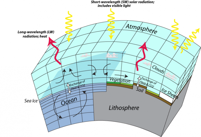
This image is a diagram illustrating the Earth's energy balance, showing the interactions between short-wavelength (SW) solar radiation and long-wavelength (LW) radiation with the atmosphere, lithosphere, and ocean. The diagram highlights the exchange of heat and CO2 across different components of the Earth system.
- Diagram Type: 3D schematic
- Components:
- Atmosphere: Top layer
- Contains clouds
- Receives short-wavelength (SW) solar radiation (yellow arrows) from the sun
- Emits long-wavelength (LW) radiation (red arrows) as heat
- Lithosphere: Bottom layer
- Includes vegetation, soil, and ice sheets
- Interacts with the atmosphere through the exchange of heat and CO2 (black arrows)
- Ocean: Middle layer
- Contains sea ice
- Shows circulation patterns (curved arrows)
- Exchanges heat and CO2 with the atmosphere (black arrows)
- Atmosphere: Top layer
- Processes:
- SW solar radiation (yellow arrows) enters the atmosphere, some reflecting off clouds
- LW radiation (red arrows) is emitted from the Earth’s surface and atmosphere
- Heat and CO2 exchange occurs between the atmosphere, lithosphere, and ocean
The diagram visually represents how solar energy drives Earth's climate system, with interactions between the atmosphere, land, and ocean influencing heat distribution and CO2 cycling.
As you can see, the models include land, air, and ocean domains, and each of these domains is treated somewhat separately since different processes act within the various domains. The more cells in a model, the closer it can approximate the real Earth, but too many cells would require more computing power than is available. The history of these models is closely connected to the history of advances in computing power, and the current generation of high-end GCMs are among the most computationally-intensive programs in existence. Models are in a continuing state of development and evolution, so in the future, they will be more complex and realistic; with continued advances in computational power and reduction in the cost of runs, models are set to take on more ambitious tasks such as making very fine projections about an ever-expanding number of environmental variables. Combine them with robots and look out!
What’s so important about these models that people would devote their careers to building and refining programs that take days to run on the fastest computers? The power and utility of these models is that they can show us how climate changes on a regional scale, which is of utmost importance in planning for our future. In our future, we are probably going to be the most effective in dealing with climate change on the scale of regions like states and countries, so having a model that shows us what those regional changes are likely to be is a very important tool.
A key aspect of using models is understanding the uncertainty of their predictions. They are simulations, after all. As you will see, most of the results are cast in terms of ranges, for instance, the temperature predictions for 2100 under the different emission scenarios are given with significant bands of uncertainty. The reading for this module is the Summary of the Intergovernmental Panel on Climate Change for Policy Makers. When you read this, you will see how scientists convey the uncertainty of model predictions.