How do GCMs Work?

How do GCMs Work?

In a highly simplified sense, the operation of GCMs can be thought of in a few basic steps.

1. Divide up the atmosphere and oceans into a complex 3-D grid; each grid may represent 2° of latitude and 2° of longitude (roughly 200 km on a side), and the models typically have 20 - 40 vertical layers, which would give you about half a million cells.
2. Assign the starting conditions for each grid — the type of material (air, soil, water, etc.), temperature, salinity of the oceans, humidity of the air, greenhouse gas concentrations, insolation, and a whole host of other variables and constants. Typically, these starting conditions are a simplified snapshot of the current climate on Earth.
3. Based on the temperature, salinity, and humidity, the program calculates the pressure in each grid cell, which combines with the rotation of the Earth to determine the velocities in each cell (see figure below). The velocities then determine how the cells will exchange heat, moisture, salinity, etc., with their neighboring cells. The program then makes all of these transfers, and then updates the conditions of each cell — these new conditions then determine how things will move in the next time step. These calculations are done in very short time increments (typically a few minutes), and the result is that they can simulate the circulation of the atmosphere and the oceans.
   

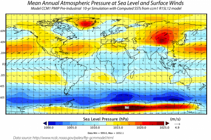   Mean Atmospheric Pressure and Winds from the NCAR GCM. The air pressure at the surface is shown in the colors — blue represents low pressure; red is high pressure. Also shown are the approximate average wind directions and strengths that would result from this map of pressure difference. The winds move from high-pressure areas to low-pressure areas, but they are bent by the Coriolis effect.

   Credit: David Bice © Penn State University is licensed under CC BY-NC-SA 4.0

   This figure comes from a run of the NCAR model, called CCM (Community Climate Model) and represents the atmospheric pressure at sea level averaged over 10 years. Also shown is the pattern of winds that results from the combination of the forces due to the pressure differences (air flows from high to low pressure, driven by a Pressure Gradient Force and the Coriolis Force, which is related to the rotation of the Earth. The length of the arrows is proportional to the strength of the winds. Note that the model produces belts of pressure that are very similar to the observed pressure belts — low pressure near the equator, high pressure at 30N and 30S, low pressure at 50-60N and 50-60S, and high pressure again near the poles, patterns we learned about in Module 3.

4. Based on temperature, pressure, flow patterns, and humidity, the models simulate the formation of clouds, which then impact the albedo (reflectance of sunlight) and the absorption of heat emitted from the surface.
5. The models also calculate the evaporation of water from the surface and the precipitation of water, and its runoff over the land back to the oceans. The evaporation and precipitation are associated with big transfers of energy, and the model keeps track of this, too.
6. All models represent land topography. Many models also include representations of photosynthesis on land, the exchange of CO² between the plants, soil, oceans, and atmosphere, and sedimentation in the ocean.