Click here to see a text description.
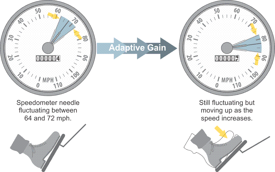
Kalman filtering is named for Rudolf Emil Kalman’s linear recursive solution for least-squares filtering. It is used to smooth the effects of system and sensor noise in large datasets. In other words, a Kalman filter is a set of equations that can tease an estimate of the actual signal, meaning the signal with the minimum mean square error, from noisy sensor measurements. Kalman filtering is used to ensure the quality of some of the Master Control Station (MCS) calculations, and many GPS/GNSS receivers utilize Kalman filtering to estimate positions. Kalman filtering can be illustrated by the example of an automobile speedometer. Imagine the needle of an automobile’s speedometer that is fluctuating between 64 and 72 mph as the car moves down the road. The driver might estimate the actual speed at 68 mph. Although not accepting each of the instantaneous speedometer’s readings literally, the number of them is too large, he has nevertheless taken them into consideration and constructed an internal model of his velocity. If the driver further depresses the accelerator and the needle responds by moving up, his reliance on his model of the speedometer’s behavior increases. Despite its vacillation, the needle has reacted as the driver thought it should. It went higher as the car accelerated. This behavior illustrates a predictable correlation between one variable, acceleration, and another, speed. He is more confident in his ability to predict the behavior of the speedometer. The driver is illustrating adaptive gain, meaning that he is fine-tuning his model as he receives new information about the measurements. As he does, a truer picture of the relationship between the readings from the speedometer and his actual speed emerges, without recording every single number as the needle jumps around. The driver’s reasoning in this analogy is something like the action of a Kalman filter. Without this ability to take the huge amounts of satellite data and condense it into a manageable number of components, GPS/GNSS processors would be overwhelmed. Kalman filtering is used in the uploading process to reduce the data to the satellite clock offset and drift, 6 orbital parameters, 3 solar radiation pressure parameters, biases of the monitoring station's clock, and a model of the tropospheric effect and earth rotational components.