The Ionospheric Effect, dion
The Earth's Ionosphere is variable
One of the largest errors in GPS positioning is attributable to the atmosphere. The long, relatively unhindered travel of the GPS signal through the virtual vacuum of space changes as it passes through the earth’s atmosphere. Through both refraction and diffraction, the atmosphere alters the apparent speed and, to a lesser extent, the direction of the signal. This causes an apparent delay in the signal's transit from the satellite to the receiver.
Ionized Plasma
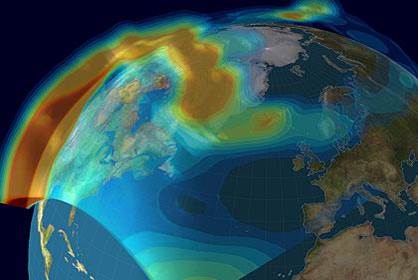
The ionosphere is ionized plasma comprised of negatively charged electrons which remain free for long periods before being captured by positive ions. It is the first part of the atmosphere that the signal encounters as it leaves the satellite. The magnitude of these delays is determined by the state of the ionosphere at the moment the signal passes through, so it's important to note that its density and stratification varies. The sun plays a key role in the creation and variation of these aspects. Also, the daytime ionosphere is rather different from the ionosphere at night.
Ionosphere and the Sun
When gas molecules are ionized by the sun’s ultraviolet radiation, free electrons are released. As their number and dispersion varies, so does the electron density in the ionosphere. This density is often described as total electron content or TEC, a measure of the number of free electrons in a column through the ionosphere with a cross-sectional area of 1 square meter: 1016 is one TEC unit. The higher the electron density, the larger the delay of the signal, but the delay is by no means constant.
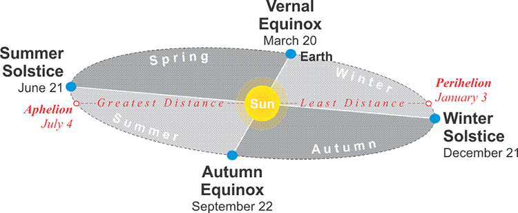
The ionospheric delay changes slowly through a daily cycle. It is usually least between midnight and early morning, and most around local noon or a little after. During the daylight hours in the midlatitudes, the ionospheric delay may grow to be as much as five times greater than it was at night, but the rate of that growth is seldom more than 8 cm per minute. It is also nearly four times greater in November, when the earth is nearing its perihelion, its closest approach to the sun, than it is in July near the earth’s aphelion, its farthest point from the sun. The effect of the ionosphere on the GPS signal usually reaches its peak in March, about the time of the vernal equinox.
Ionospheric Stratification
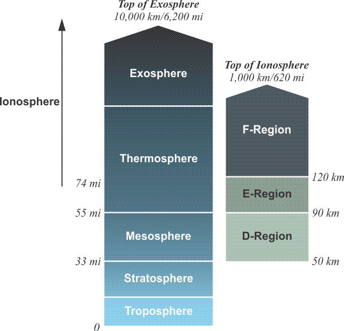
For ease of reference, the ionosphere can be said to extend from 50 kilometers to 1,000 kilometers above the earth's surface. It can be divided into the mesosphere and thermosphere, et cetera that are themselves composed of layers: D, E, and F. Neither the boundaries between these regions, nor the upper layer of the ionosphere, can be defined strictly. Here are some general ideas on the subject. The lowest detectable layer, the D region, extends from about 50 km to 90 km. It has almost no effect on GPS signals and virtually disappears at night. The E region, also a daytime phenomenon, is between 90 km and 120 km. Its effect on the signal is slight, but it can cause the signal to scintillate. The layer that affects the propagation of electromagnetic signals the most is the F region. It extends from about 120km to 1000km The F region contains the most concentrated ionization in the atmosphere. In the daytime, the F layer can be further divided into F1 and F2. F2 is the most variable. F1, the lower of the two, is most apparent in the summer. These two layers combine at night. Above, the F layer is fully ionized. It is sometimes known as the photosphere or the H region.
The ionosphere is not homogeneous and unchanging. It is in constant flux. Therefore, it's impossible to have a correction that's static. Also its behavior in one region of the earth is liable to be unlike its behavior in another. For example, ionospheric disturbances can be particularly harsh in the polar regions. But the highest TEC values and the widest variations in the horizontal gradients occur in the band of about 60° of geomagnetic latitude. That band lies 30° north and 30° south of the earth’s magnetic equator.
Satellite Elevation and Ionospheric Effect
The severity of the ionosphere’s effect on a GPS signal depends on the amount of time that signal spends traveling through it. A signal originating from a satellite near the observer’s horizon must pass through a larger amount of the ionosphere to reach the receiver than does a signal from a satellite near the observer’s zenith. In other words, the longer the signal is in the ionosphere, the greater the ionosphere’s effect on it.
Group and Phase Delay
The ionosphere is dispersive, which means that the apparent time delay contributed by the ionosphere depends on the frequency of the signal. During the signal’s trip through the ionosphere, this dispersive property causes the codes, the modulations on the carrier wave, to be affected differently than the carrier wave itself. The P code, the C/A code, the Navigation message, and all the other codes appear to be delayed, or slowed, affected by what is known as the group delay. But the carrier wave, itself, appears to speed up in the ionosphere. It is affected by what is known as the phase delay. It may seem odd to call an increase in speed a delay. It is sometimes called phase advancement. In any case, it is governed by the same properties of electron content as the group delay, phase delay just increases negatively. Please note that the algebraic sign of dion is negative in the carrier phase equation and positive in the pseudorange equation. In other words, a range from a satellite to a receiver determined by a code observation will be a bit too long and a range determined by a carrier observation will be a bit too short.
The Magnitude of the Ionospheric Effect
The error introduced by the ionosphere can be very small, but it may be large when the satellite is near the observer’s horizon, the vernal equinox is near, and/or sunspot activity is severe. For example, the TEC is maximized during the peak of the 11-year solar cycle. It also varies with magnetic activity, location, time of day, and even the direction of observation. In any case it's fair to say that one thing one can depend on is the longer that the GPS signal remains in the atmosphere, the longer its trip through that atmosphere, the greater the effect of attenuation will be. So, one of the things that a GPS receiver ought to do is ignore the signals coming from satellites that are near the observer's horizon. Obviously, as the GPS satellite is low in the sky, the signal is going through a greater atmosphere than it would be when it is directly overhead at zenith. This is one of the reasons why it's a good idea to have a mask angle on the GPS receiver (i.e.15-20 degrees) such that it will ignore the signals that are low, coming in through a great deal of atmosphere. So, no matter what time of year or the time of day, you want to avoid going through the atmosphere and get signals from satellites that are a little bit higher in the sky. It would also be a good idea to try to model the effect of the ionosphere. There's actually an aspect of GPS that allows us to have a pretty good shot at quantifying the effect of the atmosphere on our observations.
Different Frequencies Are Affected Differently
Another consequence of the dispersive nature of the ionosphere is that the attenuation for a higher frequency carrier wave is less than it is for a lower frequency wave. That means that L1, 1575.42 MHz, is not affected as much as L2, 1227.60 MHz, and L2 is not affected as much as L5, 1176.45MHz. This fact provides one of the greatest advantages of a dual-frequency receiver over the single-frequency receivers. The separations between the L1 and L2 frequencies (347.82 MHz), the L1 and L5 frequencies (398.97 MHz) and even the L2 and L5 frequencies (51.15 MHz) are large enough to facilitate estimation of the ionospheric group delay. Therefore, by tracking all the carriers, a multiple-frequency receiver can model and remove, not all, a portion of the ionospheric bias. There are now several possible combinations, L1/L2, L1/L5 and L2/L5. It is even possible to have a triple frequency combination to help ameliorate this bias.
The frequency dependence of the ionospheric effect is described by the following expression (Klobuchar 1983 in Brunner and Welsch, 1993):
Where:
As the formula illustrates, the time delay is inversely proportional to the square of the frequency; in other words, the higher the frequency, the less the delay. For example, the ionospheric delay at 1227.60 (L2) is 65% larger than at 1575.42 MHz (L1), and at 1176.45 MHz (L5) it is 80% larger than 1575.42 (L1).
Broadcast Correction
A predicted total UERE is provided in each satellite's Navigation message as the user range accuracy (URA), but it is minus ionospheric error. To help remove some of the effect of the ionospheric delay on the range derived from a single frequency receiver, there is an ionospheric correction available in another part of the Navigation message, subframe 4. However, this broadcast correction should not be expected to remove more than about three-quarters of the error, which is most pronounced on long baselines. Where the baselines between the receivers are short, the effect of the ionosphere can be small, but as the baseline grows, so does the significance of the ionospheric bias.