Prioritize...
The change in a quantity over a certain distance is called the gradient. When you've finished this page, you should be able to discuss gradients, why they're important to meteorologists, and identify / interpret relatively large and small gradients on contour maps.
Read...
Besides allowing meteorologists to estimate values of weather variables at specific points, contour maps are also useful tools that help meteorologists to see patterns in the data. In other words, contour maps make it easy for meteorologists to see how a weather variable (like temperature or pressure) is changing over a large area. Maps of isotherms allow meteorologists to identify regions of warm and cold air, as well as how temperatures change over certain areas. Similarly, maps of isobars allow meteorologists to find areas of high and low pressure, and see how pressure changes over certain areas.
The change in a variable over a certain distance is called the gradient, and gradients are very important in meteorology. Zones where weather variables have large changes are often zones of active weather, so meteorologists like to keep tabs on areas with so-called "large gradients." Tuck this idea away, as the importance of gradients will come back again and again in our studies of meteorology.
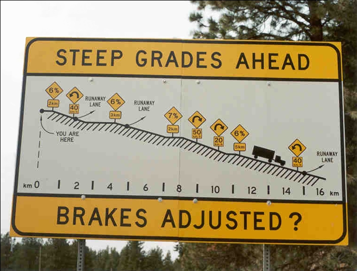
But, to start us off in our discussions of gradients, let's return to the example of elevation. Driving to the summit of the beautiful mountains in central Pennsylvania, motorists are greeted by signs that warn of "steep grades" ahead, which refers to large gradients. What does that mean in practical terms? For the mountain road to have a large gradient, the elevation of the road must change relatively rapidly over a short traveling distance. In other words, you're driving on a steep hill. Similarly, a small gradient means that the elevation of the road changes very little with distance (the road is relatively flat).
How do we distinguish between a large and small gradient on a topographical map? Let's return to the video showing the virtual topography of Hawaii (video transcript) you saw earlier. Remember that the contours of constant elevation are packed close together in areas where the elevation changes rapidly over short distances (like near the mountain summits). Thus, a large gradient on a topographical map, which marks a large change in elevation over a relatively short horizontal distance (steep terrain), corresponds to a tight packing of contours.
Meanwhile, the "packing" of contours of constant elevation is rather loose where the terrain is flatter. In other words, the gradient is small. Thus, a small gradient, which marks little change in elevation over a relatively short horizontal distance (fairly flat terrain), corresponds to a loose packing of contours.
Now let's take what we've learned from topographical maps and generalize it to weather maps. Check out the 06Z analysis of sea-level pressure on March 15, 2017 (below), which shows a powerful low-pressure system along the New England Coast. Note the tight packing of isobars over the northeastern U.S. and eastern Canada, indicating a large pressure gradient over this region (relatively large pressure changes over a short distance). As you'll learn in later in the course, tight packings of isobars (large pressure gradients) correspond to strong surface winds. This case was no exception! This area of low pressure was dubbed "The Blizzard of 2017" and winds along the coast in Massachusetts gusted to more than 70 miles per hour.
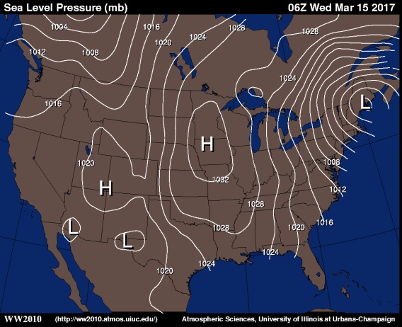
On the flip side, for an example of a small pressure gradient, look at the western United States on the map above. There's not a single isobar in California or Nevada, and overall isobars are packed very loosely in the West, so pressure changes very little over the entire region.
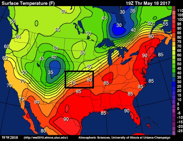
Turning our attention to temperature, tightly packed isotherms represent large horizontal changes in temperature over a relatively short distance (that is, a large temperature gradient). For example, the analysis of surface isotherms from 19Z on May 18, 2017 shows a very large temperature gradient (tight packing of isotherms) stretching all the way from the Southwestern U.S. to the Great Lakes and into Canada. Such a large temperature gradient marks a contrast between very warm air and colder air. For example, check out the change in temperature just in the state of Kansas (outlined in the black box). In the southeast corner of the state, temperatures were in the 80s. In the northwest corner, temperatures were in the 40s! As we will learn in later lessons, large temperature gradients often indicate the presence of cold and warm fronts, which you've probably heard weathercasters talk about before (and that was certainly the case here)
On the other hand, if you want to see an example of a small temperature gradient, look no further than the Gulf Coast States. The packing if isotherms was very loose, and temperatures didn't change very much with distance. In fact, temperatures over a several state area were mainly between 85 and 90 degrees.
To see another example of interpreting temperature gradients, check out the short video (1:40) showing some large and small temperature gradients in the winter time!
A useful thing that we can do with contour maps, and another one of your objectives from lesson one, is to be able to estimate and compare gradients on contour maps. So this is a map of surface temperature. And so we would be looking at temperature gradients, changes in temperature over certain distances.
And we want to look for areas of relatively large temperature gradients and relatively small temperature gradients. And where there's a large temperature gradient, that means the temperature is changing by a lot over a relatively small distance. So an example of a large temperature gradient would be over the eastern United States, say over the Appalachian Mountains, the lines are packed very close together.
That means temperature is changing by a lot over a relatively small distance. Look over here near the Ohio River, temperatures are near zero or below zero. And over to the east, along the east coast of North Carolina, temperatures are in the 40s. So temperature changes by a lot over that distance. You get a tight packing of isotherms and that's a large temperature gradient.
A small temperature gradient, on the other hand, would be where the lines are packed very loosely. We see that here along the Canadian border, North Dakota, and Minnesota. There's not a tight packing of the lines at all. That means the temperature doesn't change by very much over that distance.
So we see this minus 15 degree isotherm here. There's this closed isotherm which is minus 20 degrees. And then over here near Lake Superior there's a minus 15 degree isotherm again. So temperatures are largely between minus 15 degrees and a little bit lower than minus 20 within that circle, that closed isotherm there.
One quick note: When talking about gradients, be careful that you use the proper terminology. For example, if temperature changes rapidly over a short distance, you might refer to this as a "strong," "tight," "steep," or "large" gradient. You wouldn't, however, say that the "temperature gradient is changing rapidly." Doing so means that the change in temperature is changing. While this is certainly possible, it's not how we talk about a single gradient, because the gradient itself IS the change over a certain distance.
The bottom line is that meteorologists really pay attention to gradients in temperature and pressure (among other variables), mainly because large gradients can be zones of very "interesting" weather! Before wrapping up the lesson, make sure you try your hand at the Key Skill section below, to make sure you can "size up" gradients.
Key Skill...
After studying this section, you should be able to identify and describe gradients based on contour maps. You should be able to look at a location on a contour map and describe a gradient as relatively large or small compared to other locations on the map, and be able to describe what that means for changes in the variable (is it changing by a lot or by a little?).
Try these examples out for yourself. For each example, use the image below...
Compare the magnitudes of the temperature gradients at stations A and B. For example, which station has the larger gradient? How do you know? Are the gradients large or small compared to other locations on the map?
Answer: Station A has a larger gradient than Station B. We know this because the isotherms are packed closer together at A than at B. Alternatively, we could say that over a fixed distance near Station A (say, 1 cm on the map), the temperature changes a great deal more than for the same distance at Station B. While Station A shows a large gradient, there are perhaps slightly larger gradients in temperature in South Carolina and northern Canada. Station B's temperature gradient is certainly among the smallest on the map.
Example #2:
Perform the same analysis that you did in Example #1, but with stations C and D.
Answer: Station C has a larger gradient than Station D. We know this because the isotherms are packed closer together at C than at D. We could also say that over a fixed distance near Station C (say, 1 cm on the map), the temperature changes a great deal more than for the same distance at Station D. Station C shows one of the largest gradients on the map. Station D's temperature gradient is certainly among the smallest on the map.