Playing Weather on the Computer: Making a "Mesh" out of Things
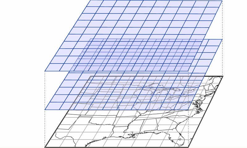
For U.S. forecasters, the “board” used for “playing the game” of NWP is typically North America and adjacent oceans. Like a chess board, this geographical arena can be neatly divided into a mesh of regularly spaced points called a grid. For the record, these grid points are the locations at which the computer calculates the numerical forecast (meteorologists refer to this type of model as a grid-point model). The spacing between grid points varies from grid-point model to grid-point model (and sometimes even within a single model). Some grid-point models have a "coarse" mesh, with large spacing between relatively few grid points. Other grid-point models are "fine" mesh, with a small spacing between relatively many grid points. Whether the mesh of grid points is coarse or fine ideally governs the quality of the forecast (we'll explore this idea in just a moment).
Mimicking a game of three-dimensional chess, there are also meshes of regularly spaced points at specified altitudes, stacking from the ground to the upper reaches of the atmosphere (see the figure below). Thus, a three-dimensional array emerges that covers a great volume of the atmosphere, ready to be filled with weather data at each grid point. The typical horizontal spacing of grid points for operational computer models is typically on the order of ten kilometers. The vertical spacing of grid points varies from tens to hundreds of meters.
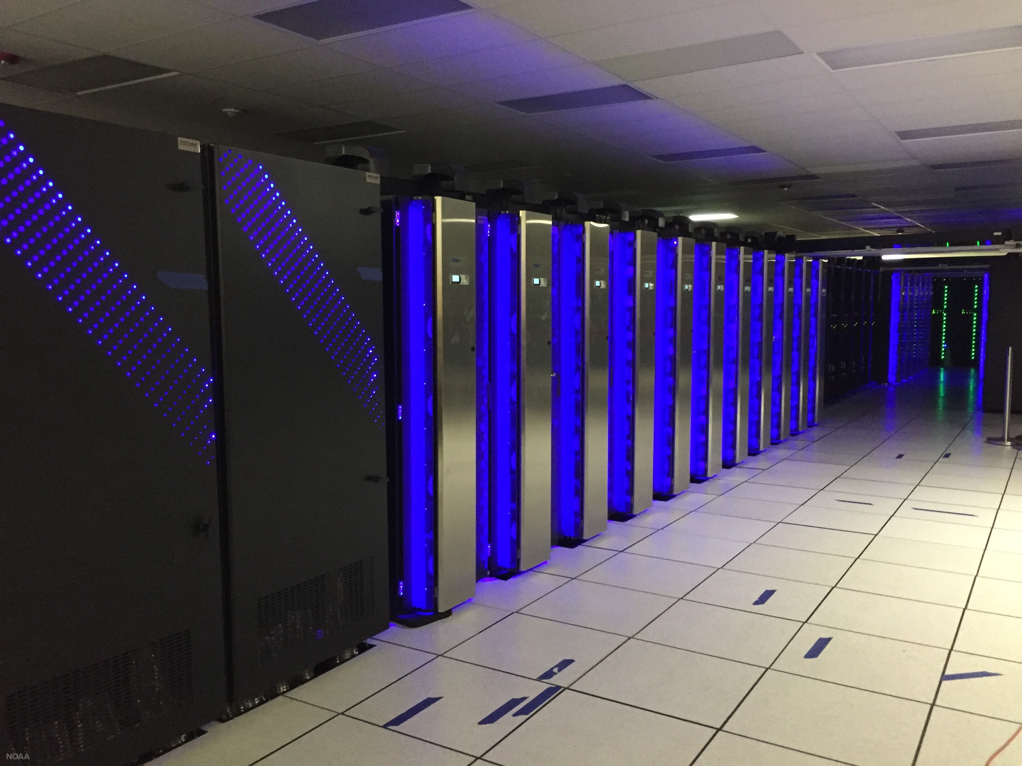
Once a simulation (sometimes called a "model run" or just plain “run”) has begun, the computer predicts (calculates) the values of moisture, temperature, wind, and so on, at each grid point at a future time, typically a few virtual minutes into the future. To perform this feat, powerful, high-speed supercomputers make trillions to quadrillions of calculations each second (see photograph farther down on the page). Thereafter, the computer calculates the same parameters for the next forecast time (a few more minutes into the future), and so on. For a short-range prediction, this "leapfrog time scheme" typically ends 84 hours into the virtual future, taking on the order of an hour of real time to complete.
Even leap-frogging just a few virtual minutes into the future is fraught with error because the computer makes calculations for one time and then “leaps” to make calculations a few more virtual minutes later, skipping calculations for intermediate times between the starting and ending points of the leap. Like taking short cuts while solving a complicated algebra problem, skipping steps inevitably leads to errors.
This sacrifice in accuracy is a gambit with which forecasters must live. They could, theoretically, make a more accurate computer forecast by reducing the size of the time interval in the leapfrog scheme. However, a smaller time interval would require faster and more powerful computers to support the increased computational load. Also, meteorologists could increase the number of grid points to improve forecasts with the hope that smaller grid spacings could better capture smaller-scale weather phenomena. But such a scheme also demands faster and faster supercomputers. Though technology continues to advance, there is a practical limit to what computers can do, so there will never be a perfect computer forecast. Never.
Another shortcoming of computer guidance results from the way each simulation is initialized. By initialization, we mean the mathematical scheme used to represent the state of the atmosphere at the time the computer simulation begins. In other words, to initialize a model means to assign appropriate values of pressure, temperature, moisture, wind, and so on, to each grid point before the leapfrog scheme begins. These values typically come from both observations and previous forecasts.
Another complication arises in grid-point models because the grid points don’t necessarily fall directly on the locations where weather observations are routinely taken. In addition, the observations themselves have deficiencies: Instrument error is unavoidable, and the observational network, particularly over the oceans, has many gaps. As a result, the best “first guess” for the initialization is often a forecast from the previous model run. This first guess is then adjusted by incorporating real weather observations, taken both at the surface and aloft. Weather-balloon-toted radiosondes take upper-air measurements at 00 UTC and 12 UTC each day, so these are typically the times at which computer runs are initialized (short-range models are also initialized at 06 UTC and 18 UTC). By way of example, the “first-guess” initialization for a model initialized at 12 UTC might be the 12-hour forecast from the previous 00 UTC run. Though the complicated process of initialization is imperfect, it’s the best meteorologists can do to produce the starting values for a computer simulation.
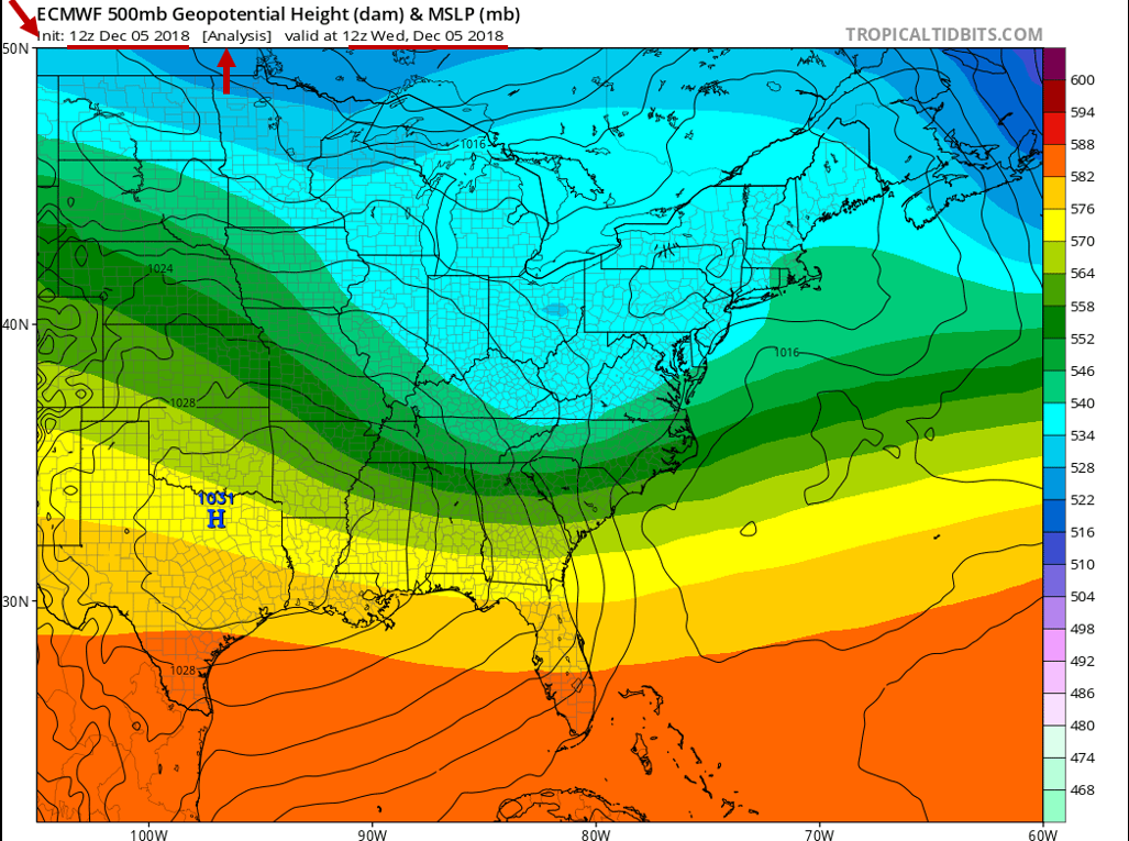
In practice, the initialization is sometimes referred to as the 0-hour forecast or the model analysis. Below is the initialization / 0-hour forecast / model analysis (whichever term you prefer) of a computer simulation that was run at 12 UTC on December 5, 2018. This chart represents the model's best representation of the current state of the atmosphere at 12 UTC on December 5, 2018. For the record, this initialization shows mean sea-level isobars (thin, black contours) and 500-mb heights (color-coded in dekameters). Again, any errors in this representation will be magnified as the simulation proceeds in time.
Worldwide, there are many different computer models run on a day-to-day basis that provide guidance for weather forecasters. The various models differ in their geographical area, initialization technique, representation of topography, mathematical formulation, length of forecast (in other words, how far into the future they are run), and other factors.
In 2011, the NEMS NMM-B became the flagship grid-point model that U.S. meteorologists use for short-term weather forecasts. NOAA is big on acronyms, and NEMS stands for NOAA Environmental Modeling System, which is the super-framework within which the National Centers for Environmental Prediction (NCEP) in Washington, DC, initializes, runs, and post-processes its suite of computer models. NMM-B is the Non-Hydrostatic Multiscale Model based on a "B staggering in the horizontal." Don't get nervous. Without getting too complicated here, "B-staggering in the horizontal" means that the predicted north-south and east-west components of the wind lie on the four corners of each grid cell. All other forecast variables (temperature, pressure, vertical motion, etc.) lie in the center of the cell. Yes, it's inside baseball, and you really don't need to know such details, but we at least wanted you to have a sense for what the "B" in "NMM-B" means.
Let's just drop all the formality here and call the NEMS NMM-B the NAM, which is short for the North American Model (now that's an acronym we can live with). For the record, the NAM has a horizontal grid spacing of 12 kilometers (though some versions of the model run with a horizontal grid spacing of 4 kilometers). NCEP runs the NAM four times a day at 00 UTC, 06 UTC, 12 UTC and 18 UTC. The NAM produces numerical weather forecasts out to 84 hours into the future.
A few years prior to October 18, 2011, the Weather Research and Forecasting Model (WRF, for short) served as the North American Model. The only reason we point this out to you is that you'll see "WRF" labeled on some of the progs we present as case studies in this chapter. Don't get nervous. All the concepts you'll learn about interpreting NAM progs are universal (they apply to both the old WRF and the newer NEMS NMM-B).
Another example of a grid-point model used by U.S. weather forecasters is the High-Resolution Rapid Refresh (HRRR) model, which has a horizontal grid spacing of 3 kilometers and produces a new 18-hour forecast every hour.
We'll talk more about the NAM later in the chapter. For now, we want to introduce another numerical weather prediction model called the Global Forecast System (GFS), which NCEP runs daily at 00 UTC, 06 UTC, 12 UTC and 18 UTC. As it turns out, the GFS is not a grid-point model. Let's investigate.