More on Ensemble Forecasting: Spaghetti Plots
Computer forecasts can go awry for several reasons. Right off the bat, numerical weather predictions can "bust" pretty quickly if the model is initialized poorly - in other words, if it does not reasonably represent the current state of the atmosphere. Even "good" initializations have flaws, so they never quite represent the current state of the atmosphere with perfect accuracy. Either way, uncertainty in varying degrees is almost always introduced into numerical weather prediction, and this uncertainty grows with increasing forecast time.
As you learned earlier, meteorologists compensate by implementing a technique called ensemble forecasting, which gauges the sensitivity of a computer model's prediction to the way it's initialized. Specifically, meteorologists make minor changes to the initialization of a lower-resolution version of a specified operational model called the control member. For example, the control member in the GEFS has lower resolution than the operational GFS model. At any rate, the control member is run using this slightly different initial state. Then meteorologists tweak the initialization of the control member yet another time, in a slightly different way, and run the control member again using this new initial state. This process of "tweaking" the initial conditions of the control member is repeated a number of times (for some models, several dozen times), yielding a set of ensemble members.
If all or most of the ensemble members come up with basically the same numerical prediction for a specific forecast day, meteorologists have a relatively high degree of confidence in that day's forecast. If, however, the tweaked model runs predict several noticeably different scenarios for the day in question, then forecasters have a fairly low degree of confidence in the numerical prediction.
In our previous introduction to short-range ensemble forecasts, we examined the Blizzard of January 25-28, 2015, and showed you the efficacy of short-range ensemble forecasting technique, especially when there's a high degree of uncertainty in the forecast. Revisit the image above and focus your attention on the spread in the ensemble forecasts for the western edge of snowfall equal to ten inches. This spread indicated high uncertainty for short-range predictions of heavy snowfall on the western flank of the nor'easter. Such a spread of contours almost looks like spaghetti noodles, assuming you let your imagination run a bit wild. Hold this "pasta" thought for a moment.
To investigate the role of "spaghetti," forecast uncertainty, and ensemble forecasting in medium-range predictions, let's shift away from winter weather and take a look at a case from the field of tropical weather forecasting. We will focus our attention on Hurricane Michael, which made landfall on October 10, 2018, near Mexico Beach on the panhandle of Florida as a high-end Category-4 hurricane (see the 4.5-hour loop of visible images from GOES 16 below). Maximum sustained winds were 155 mph and the minimum pressure in the eye was 919 mb. These two images show the catastrophic damage produced by storm surge and wind at Mexico Beach: (Image #1, Image #2).
One of the tools that tropical forecasters sometimes use is a multi-model ensemble system to predict the track of tropical cyclones in both the short and medium range. In tropical forecasting, this multi-model approach sometimes includes three ensemble prediction systems. As you already learned, the GFS model has an ensemble prediction system called the Global Ensemble Forecast System (GEFS). The Canadian Modeling Centre has an ensemble prediction system called the Canadian Global Ensemble Prediction System (GEPS). The U.S. Navy also has an ensemble prediction system based on their own model, the Navy Global Environmental Model (NAVGEM).
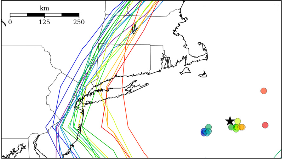
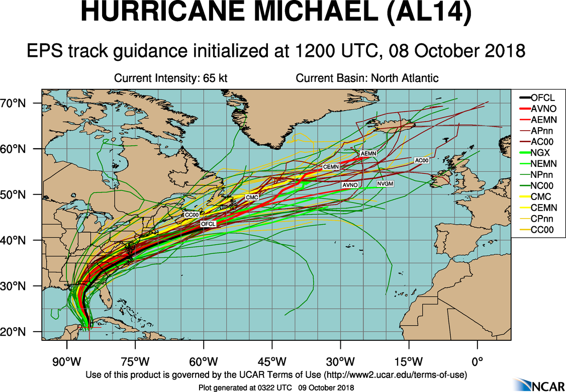
When Hurricane Michael threatened the Gulf Coast, forecasters likely looked at a multi-model ensemble system that incorporated all three of the above ensemble prediction systems (see example below). These forecast tracks were based on the 12 UTC run on October 8, 2018, of these three ensemble prediction systems. You can interpret the color coding as follows: red = GEFS (the GFS ensemble prediction system), yellow = GEPS (the Canadian EPS), and green = NAVGEM EPS (from the U.S. Navy). The black track corresponds to the National Hurricane Center's official forecast track. This ensemble display of possible predicted tracks for Hurricane Michael includes the mean ensemble forecast from each of the three ensemble prediction systems, the control members of the GEFS, GEPS, and the NAVGEM EPS, and the deterministic forecast by each of the operational models. Looks like a bunch of spaghetti noodles, wouldn't you say?
With regard to medium-range forecasting, meteorologists along the Middle Atlantic Coast, for example, would have used this multi-model approach. Why would these forecasters incorporate this multi-model EPS in their process for preparing their medium-range forecast? Research has shown that a multi-model ensemble is usually more useful than a single ensemble, even if some of the ensemble members have lower skill. In the medium range, the GEFS, for example, tends to be underdispersive.
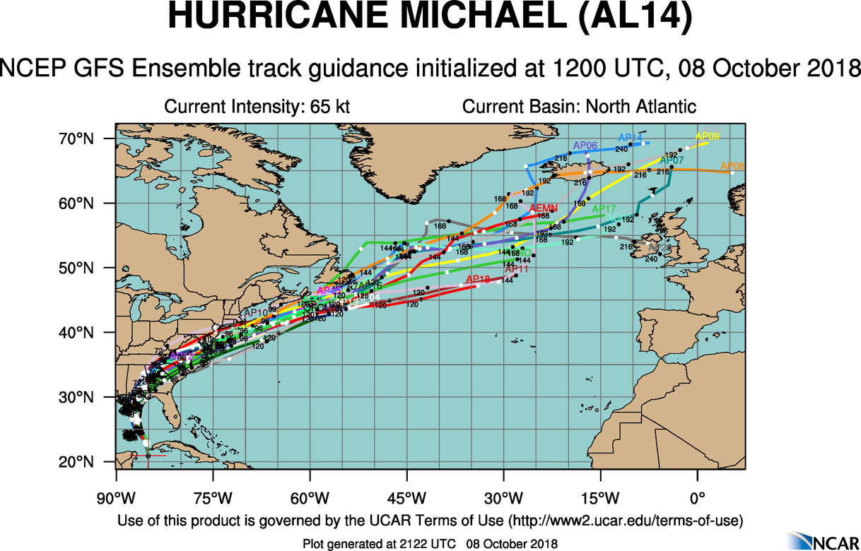
What does this mean? In the context of the predicted tracks of tropical cyclones, the spread in the forecasts is often suspiciously too small (this can occur in both in the short and medium range). You can see what we mean by looking at the GEFS track forecast for Hurricane Michael (below; larger image) and comparing its spread to the spread in the multi-model ensemble system shown above (please note that the GEFS was run at the same time as the multi-model EPS: 12 UTC on October 8, 2018). The bottom line here is that having all three ensemble forecast systems (including the GEFS) plotted on the same chart allows forecasters to see other possibilities that the GEFS might not be picking up on. Multi-model ensemble forecasts are another tool that meteorologists consult to gain insight into future tracks of tropical cycones and to help them establish the cone of uncertainty.
Of course, ensemble forecasting has more routine applications than pinning down the the possible tracks for major hurricanes. Indeed, weather forecasters use ensemble forecasting on a day-to-day basis to gauge the uncertainty of weather patterns for medium-range (and, of course, short-range) prediction. For example, forecasters will look an the ensemble forecasts for specific 500-mb heights in order to assess the uncertainty of regional medium-range forecasts.
To illustrate our point, check out the 24-hour GFS ensemble forecast (below) for the 5760-meter 500-mb height line (21 different members in blue) and 5940-meter 500-mb height line (21 different members in red) over Europe from the 00 UTC run on August 6, 2009. During summer, a 500-mb height of 5760 meters typically marks the southern edge of the relatively fast" 500-mb westerlies, while heights above 5940 meters typically correspond to hot weather. On the ensemble forecast below, the more northern green contour represents the average position of the 5760-meter height at that time of year, while the more southern green contour marks the average position of the 5940-meter height line. Having the climatological positions of these heights helps meteorologists to gauge whether heights are forecast to be above or below average at this time of year.
Given that this is only a 24-hour forecast, it's not surprising that there was a high degree of confidence with the predicted position of the 5760-meter height line (and the general 500-mb pattern) over Europe (the blue lines are pretty much in agreement). With a ridge over Scandinavia and much of central Europe, for example, a pattern of generally warmer-than-average, dry weather seemed likely over the region at the forecast time. There was a bit more uncertainty associated with the closed 5940-meter contour over northern Africa, but any slight shift in the position of this rather stagnant 500-mb high would not have much impact on the weather pattern over northern Africa; it was going to be hot no matter what!
Okay, now let's look at the 168-hour GFS ensemble forecast from the same run (see below). Look at all those lines! Is it any wonder why some meteorologists call such a graphical depiction of an ensemble forecast a spaghetti plot? Looks like they would have to use their "noodles" to figure out the forecast! Indeed, there was clearly more uncertainty in the forecast, as you would expect from a 168-hour forecast. There were even a few blue lines south of the climatological position of the 5760-meter height, suggesting cooler-than-average weather over central Europe - but these were the exception, rather than the rule. Eyeballing the mean ensemble forecast (the average position of the 21 members), you might conclude that there would be warmer-than-average weather over northern Europe around the forecast time, given that a lot of blue lines are north of the climatological position of the 5760-meter height. Meanwhile, the 168-hour GFS ensemble forecast suggested that it would get warmer over Spain (compared to the 24-hour ensemble forecast) . But how much warmer? Those red lines, representing ensemble forecasts for the 5940-meter height, are all over the place (lots of spaghetti), with a few lines never really making it to Spain. To complete our story, here's the animation of this GFS ensemble forecast out to 360 hours. Note how the uncertainty associated with the predicted position of the 5760-meter height grows with time.
We note that the European Centre for Medium-Range Weather Forecasting runs an ensemble version of its medium-range model, known as the Ensemble Prediction System (EPS). The EPS has 51 ensemble members and produces 15-day forecasts twice a day, initialized at 00 UTC and 12 UTC. Unlike the suite of ensemble forecasts produced by NCEP, the entire set of EPS forecasts is generally not available for free to the public.
As computational power has dramatically increased, the ensemble approach has also been applied to short-range forecasting (we already discussed SREF in the context of the Blizzard of January 25-28, 2015). As you learned in our introduction to ensemble forecasting, the ensemble approach provides weather forecasters with a way to gauge the sensitivity of short-range forecasts to small changes in initial conditions. Most of the time, the SREF mean forecast (the average forecast derived from the 26 SREF members) provides a reasonable starting point for meteorologists to hone their predictions. The bottom line here is that ensemble forecasting is revolutionizing the way meteorologists use computer models, both in the short range and medium range.
What about forecasts beyond the medium range, at monthly and even seasonal time scales? Research has shown that the medium-range forecasting models lose any hint of skill after approximately two weeks; in other words, to return to one of our original metaphors, the line of people becomes so long that the message of the original whisper is too twisted and mangled to be trusted. Yet the National Weather Service and many private forecasting companies routinely issue monthly and even seasonal forecasts. Let's see how they do it.