
A Simple Analogy
We're going to take a step backwards for a second and think about a much simpler system, but one that has some things in common with the global carbon cycle. First, however, we need to recognize that the natural carbon cycle is something that always varies a bit, but it has some important feedbacks in it that tend to make it stable or steady. And then, along come humans, burning an impressive amount of fossil fuel and creating a new flow in the carbon cycle. To get a sense of how a system with a tendency to remain in a steady state might respond to a new flow, we turn to a simpler model.
Our simple model is a water tub with a drain and two faucets.
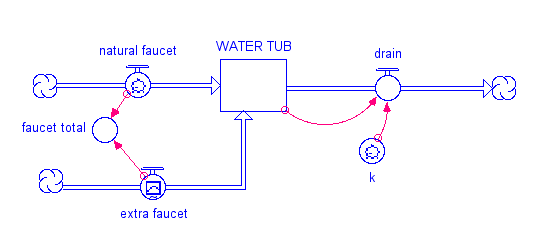
This image is a diagram titled "WATER TUB," illustrating a simplified model of a water tub system with inflows and outflows, analogous to a dynamic system reaching a steady state. The diagram uses arrows and labels to show the flow of water into and out of the tub, with a caption explaining the specific model parameters and outcomes.
- Diagram Type: Flow diagram
- Components:
- Water Tub: A central rectangular box labeled "WATER TUB," representing the reservoir of water.
- Inflows:
- Natural Faucet: An arrow labeled "natural faucet" entering the tub from the left, representing a constant water inflow.
- Extra Faucet: Another arrow labeled "extra faucet" entering the tub from the left, contributing additional inflow.
- Faucet Total: A circular node labeled "faucet total" where the natural and extra faucet inflows combine before entering the tub.
- Outflow:
- Drain: An arrow labeled "drain" exiting the tub to the right, leading to a circular node with a "k" (likely a rate constant) and then to a cloud-like symbol, indicating water leaving the system.
- Feedback:
- A red dashed arrow loops from the drain back to the tub, suggesting the drain rate is dependent on the amount of water in the tub.
- Annotations:
- The diagram does not include numerical values or scales directly on the components, but the caption provides specific parameters.
- Caption:
- "This graph shows the model results from a case where the initial amount of water in the tub was 10 liters and the faucet rate was 3 liters per time unit. The initial drain flow rate is just 10% of the starting amount of water -- 1 liter per time unit -- so the amount of water in the tub increases until it reaches 30 liters, at which point the drain flow rate is 3 liters per time unit, the same as the faucet rate. When the faucet (inflow) rate is equal to the drain (outflow) rate, the system is in a steady state. The figure also shows how the response time is defined for this kind of a system that evolves into a steady state."
The diagram visually represents a dynamic system where water accumulates in the tub until the inflow (3 liters per time unit from the faucet) equals the outflow (drain rate, which increases to 3 liters per time unit when the tub reaches 30 liters), achieving a steady state. The red dashed feedback loop indicates that the drain rate depends on the water volume, illustrating the system's response time to reach equilibrium.
One faucet represents the natural addition of water to the tub, while the other represents a new flow. The tub has a drain in it, and it takes out 10% of the water in a given time interval (the value of k is 0.1 and the drain flow is just the amount in the tub times k). When you first open the model, the extra faucet is set to zero, and if you run the model you will see that it is in a steady state — the faucet and drain are equal, so the amount in the reservoir remains constant. What happens to the system if you increase the faucet flow using the upper knob to the right of the graph? If the faucet flow increases, then at first it will be greater than the drain and the amount in the tub will increase; but as faucet flow increases, so will the drain flow, and it will eventually become equal to the faucet flow and the system will return to steady state, but one with more water in the tub. Give it a try, and see what happens. At steady state, you can write a simple equation that says:
It turns out that the response time for this system is just 1/k. In this example model, k = 0.1 so the response time is 10 time units (the units depend on how the flows are given — liters per second or minute). This response time is not the length of time required for the system to get into a steady state — it is the time required to accomplish 63%, or the change to the new steady state. Why 63%? There is some math behind this choice, but in essence, it is just a convention that helps us avoid the problem of picking the time when steady state is achieved, which is difficult since it does so asymptotically. The figure below shows how this looks. In the graphs below, the blue line for the water tub is hidden beneath the red curve of the drain — these have different scales on the left hand side, but they are the same exact shape, so one plots over the other.
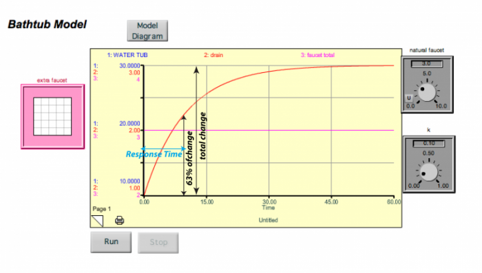
This image is a screenshot from a "Bathtub Model" simulation, depicting the dynamics of water accumulation in a tub based on inflow and outflow rates. The interface includes a graph showing the model's output, a diagram of the system, and controls for running the simulation. The caption is not provided, so I will describe the image based on its visual content.
- Interface Title: Bathtub Model
- Components:
- Graph (Center):
- Title: Model Diagram
- X-Axis: Time (unitless, range: 0 to 60)
- Y-Axis: Volume of water in the tub (liters)
- Range: 0 to 30 liters
- Data Representation:
- Red line labeled "WATER_TUB": Shows water volume starting at 10 liters, rising to a steady state of ~30 liters around time 45
- Pink dashed line labeled "% change": Indicates the percentage of total change in water volume, reaching ~63% around time 15 (labeled "Response Time")
- Horizontal pink line at 30 liters marks the steady-state volume
- System Diagram (Top Right):
- Elements:
- Natural Faucet: A control knob set to 3.0 liters per time unit (range: 0 to 5)
- Faucet Total: A node combining inflows, set to 3.0 liters per time unit
- Drain: A control knob labeled "k" set to 0.10 (range: 0 to 1), representing the drain rate constant
- Connections:
- Arrows show water flow from Natural Faucet to Faucet Total to WATER_TUB
- Feedback loop from WATER_TUB to Drain, indicating the drain rate depends on the tub's water volume
- Elements:
- Extra Faucet (Top Left):
- A pink square with a grid, labeled "extra faucet," set to 0.0 liters per time unit (range: 0 to 2)
- Controls (Bottom):
- Buttons labeled "Run" and "Stop" for controlling the simulation
- Page indicator: "Page 1"
- Additional Settings (Left):
- WATER_TUB initial value: 10 liters (range: 0 to 30)
- Time step: 0.25 (range: 0 to 2)
- Response Time: 3 (not adjustable)
- Graph (Center):
The image illustrates a dynamic system where water enters the tub at a constant rate (3 liters per time unit) and drains at a rate proportional to the water volume (k = 0.1). The graph shows the water volume increasing from 10 liters to a steady state of 30 liters, with the response time (time to reach ~63% of the total change) marked at approximately 15 time units. The simulation interface allows users to adjust parameters like faucet rates and observe the system's behavior.
I changed the faucet here to 3, and the water in the tub rose until it reached a value of 30, where the drain value then became equal to the faucet value and the system reached a new steady state. As shown by the blue arrow above, this takes 10 time units to accomplish 63% of the change.
So, this is a system that has negative feedback (the drain) that drives it to a steady state, which means that regardless of the values of the faucet or the drain constant, k, the system will find a steady state.
Now, look at what happens if we turn on a new faucet — add a new flow to a system that is in a steady state. In the figure below, you see what happens if we turn the extra faucet on for a bit and then turn it off.
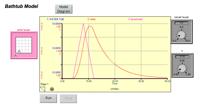
The screen presents a "Bathtub Model" simulation interface, designed to illustrate water flow dynamics in a bathtub over time. The interface includes a title "Bathtub Model" with a "Model Diagram" button at the top. A central graph features a time axis (0 to 60 units) and a volume axis (0 to 18,000 units), displaying a pink "1: WATER_TUB" curve peaking at 16,000 units around 15 time units and an orange "2: drain" curve peaking slightly later, both declining to zero. A pink "extra faucet" diagram with a faucet symbol pointing to a square labeled "1" is on the left. On the right, dials for "faucet_total" (5.0, range 0-10) and "k" (0.10, range 0-1.00) are shown. At the bottom, "RUN" and "STOP" buttons and a "Page 1" label complete the layout.
- Bathtub Model Interface
- Title: Bathtub Model
- Button: Model Diagram
- Graph
- X-axis: Time (0 to 60 units)
- Y-axis: Volume (0 to 18,000 units)
- Curves:
- Pink curve: Labeled "1: WATER_TUB"
- Peaks at ~16,000 units at 15 time units
- Declines to zero
- Orange curve: Labeled "2: drain"
- Peaks slightly after pink curve
- Declines to zero
- Pink curve: Labeled "1: WATER_TUB"
- Left Diagram
- Label: extra faucet
- Content: Flowchart with faucet symbol pointing to a square labeled "1"
- Color: Pink
- Right Dials
- Faucet_total
- Value: 5.0
- Range: 0 to 10
- k
- Value: 0.10
- Range: 0 to 1.00
- Faucet_total
- Bottom Controls
- Buttons: RUN, STOP
- Label: Page 1
The system gets thrown out of its steady state temporarily, but returns to the original steady state when the extra faucet is turned back off. Note that there is a lag time here — the water tub peaks about 5 time units after the faucet peaks (this is the sum of the two faucets). If we were to decrease k, then the response time would lengthen, and the lag time would also lengthen. Think of this spike in the extra faucet as being equivalent to a short-term addition of CO2 into the atmosphere. But what if we turn the extra faucet on and then leave it on for some time at a steady rate? This might be equivalent to us adding CO2 to the atmosphere and then keeping those emissions constant (sometimes referred to as the "stabilization" of emissions). We can simulate this scenario with our simple model, and the results are shown below.
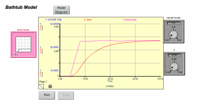
The screen displays a "Bathtub Model" simulation interface for visualizing water flow dynamics, updated with new parameters compared to the previous image. The title "Bathtub Model" is at the top with a "Model Diagram" button. A central graph plots time on the x-axis (0 to 60 units) and volume on the y-axis (0 to 40,000 units), showing a pink curve labeled "1: WATER_TUB" that rises steadily to around 30,000 units by 60 time units, and an orange curve labeled "2: drain" that increases more gradually to about 5,000 units. On the left, a pink "extra faucet" diagram shows a faucet symbol pointing to a square labeled "1." On the right, dials show "faucet_total" at 5.0 (range 0-10) and "k" at 0.50 (range 0-1.00). At the bottom, "RUN" and "STOP" buttons are present, with the interface labeled "Page 1."
- Bathtub Model Interface
- Title: Bathtub Model
- Button: Model Diagram
- Graph
- X-axis: Time (0 to 60 units)
- Y-axis: Volume (0 to 40,000 units)
- Curves:
- Pink curve: Labeled "1: WATER_TUB"
- Rises steadily to ~30,000 units by 60 time units
- Orange curve: Labeled "2: drain"
- Increases gradually to ~5,000 units by 60 time units
- Pink curve: Labeled "1: WATER_TUB"
- Left Diagram
- Label: extra faucet
- Content: Flowchart with faucet symbol pointing to a square labeled "1"
- Color: Pink
- Right Dials
- Faucet_total
- Value: 5.0
- Range: 0 to 10
- k
- Value: 0.50
- Range: 0 to 1.00
- Faucet_total
- Bottom Controls
- Buttons: RUN, STOP
- Label: Page 1
What you see is that the system responds by increasing the water in the tub until a new steady state is reached. The length of time needed to achieve the new steady state is determined by the response time of the system, which again, is governed by the magnitude of the drain constant, k.
In the real carbon cycle, this response time is measured in tens of thousands of years. For example, remember that the residence time of the deep ocean is about 3,800 years. The response time of the whole carbon cycle must be much longer than this because CO2 emissions are cycled through more than just the deep ocean. Unfortunately, you can't add up the residence time of the individual reservoirs to get the response time of the whole carbon cycle which is really what we want to know, the system is much more complex than this. The natural carbon cycle will find a new steady state (it will "stabilize") in response to our carbon emissions, but it will take many thousands of years to do so. In the meantime, the system will continue to change as it makes this adjustment.