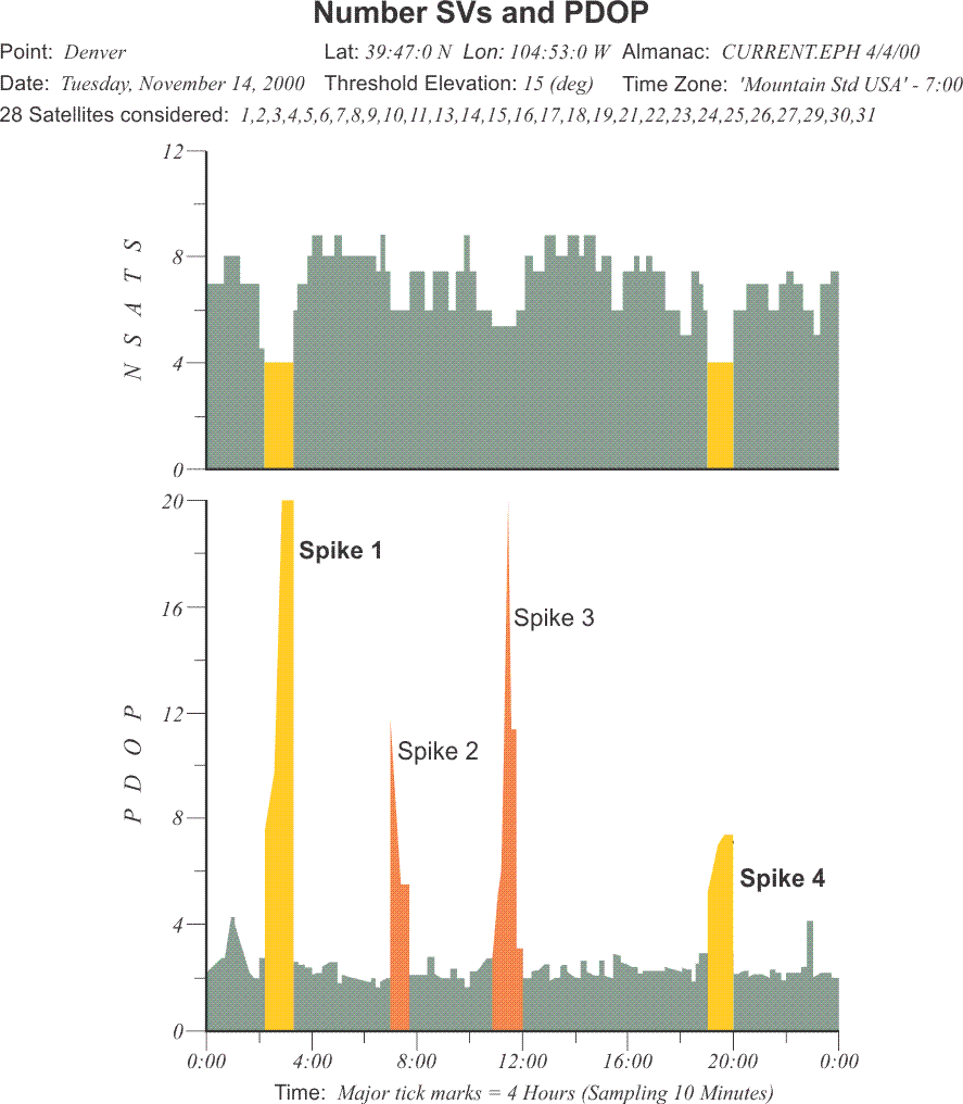
Though much of the preliminary work in producing the plan of a GPS/GNSS survey is a matter of estimation, some hard facts must be considered, too. For example, the number of GPS/GNSS receivers available for the work and the number of satellites above the observer’s horizon at a given time in a given place are two ingredients that can be determined with some certainty. Most GPS/GNSS software packages provide users with routines that help them determine the satellite windows, the periods of time when the largest numbers of satellites are simultaneously available. Today, observers are virtually assured of 24-hour coverage; however, the mere presence of adequate satellites above an observer’s horizon does not guarantee collection of sufficient data. Therefore, despite the virtual certainty that at least 4 satellites will be available, evaluation of their configuration as expressed in the position dilution of precision (PDOP) is still crucial in planning a GPS/GNSS survey. Satellites need to be available for observation at the occupied points. The same satellites need to be visible at both ends of the vectors that are going to be occupied. Most GPS/GNSS software packages allow you to know how many satellites are above a horizon at a particular location. The position dilution of precision (PDOP) is also something that needs to be taken into account in a static GPS/GNSS survey design. Here are some charts that indicate how PDOP can be evaluated in some cases. You see here the number of satellites on the left. On the right, you see the position dilution of precision. It spikes when the number of satellites drops, when some set. When there are only four, the PDOP goes way up. The geometry of the satellites from the receiver's point of view is not optimal. There are some other spikes, too, as the satellites move from one configuration to another. It is not wise to do GPS/GNSS observations when the PDOP is high. You need to be aware of those times so that in planning the observation schedule, you’re not trying to measure baselines when the PDOP is spiking.
Position Dilution of Precision (PDOP)
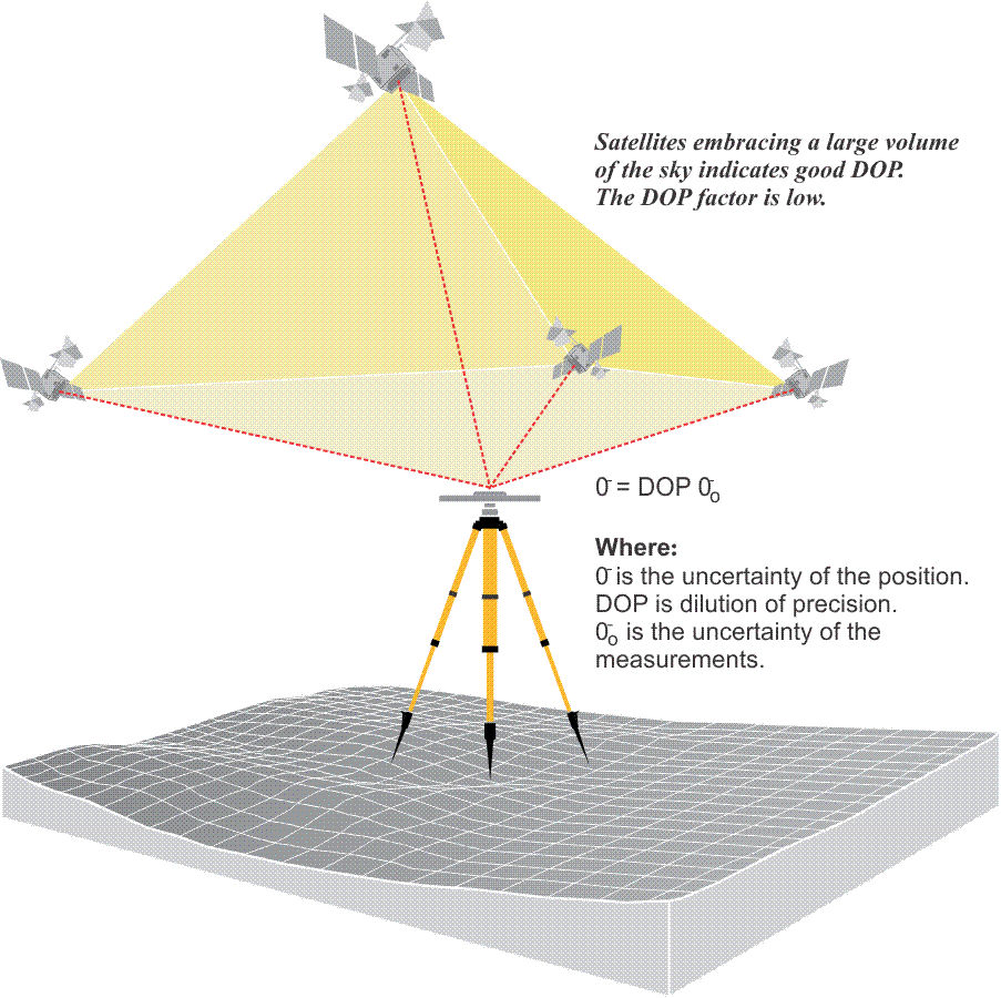
The assessment of the productivity of a GPS/GNSS survey almost always hinges, in part at least, on the length of the observation sessions required to satisfy the survey specifications. The determination of the session’s duration depends on several particulars, such as the length of the baseline and the relative position, that is the geometry, of the satellites, among others. Generally speaking, the larger the constellation of satellites, the better the available geometry, the lower the positioning dilution of precision (PDOP), and the shorter the length of the session needed to achieve the required accuracy. For example, given 6 satellites and good geometry, baselines of 10 km or less might require a session of 45 minutes to 1 hour, whereas, under exactly the same conditions, a baseline over 20 km might require a session of 2 hours or more. Alternatively, 45 minutes of 6-satellite data may be worth an hour of 4-satellite data, depending on the arrangement of the satellites in the sky. Stated another way, the GPS/GNSS receiver’s position is derived from the simultaneous solution of vectors between it and the constellation of satellites above the observer’s horizon. The quality of that solution depends, in large part, on the distribution of those vectors. For example, any position determined when the satellites are crowded together in one part of the sky will be unreliable, because all the vectors will have virtually the same direction. Fortunately, a computer can predict such an unfavorable configuration if it is given the ephemeris of each satellite, the approximate position of the receiver, and the time of the planned observation. Provided with a forecast of a large PDOP, the GPS/GNSS survey planner should consider an alternate observation plan. On the other hand, when one satellite is directly above the receiver and three others are near the horizon (but not too close) and 120° in azimuth from one another, the arrangement is nearly ideal for a 4-satellite constellation. The planner of the survey would be likely to consider such a window. However, more satellites would improve the resulting position even more, as long as they are well distributed in the sky above the receiver. In general, the more satellites, the better. For example, if the planner finds 8 satellites will be above the horizon in the region where the work is to be done and the PDOP is below 2, that window would be a likely candidate for observation. There are other important considerations. The satellites are constantly moving in relation to the receiver and to each other. Because satellites rise and set, the PDOP is constantly changing. Within all this movement, the GPS/GNSS survey designer must have some way of correlating the longest and most important baselines with the longest windows, the most satellites, and the lowest PDOP. Most GPS/GNSS software packages, given a particular location and period of time, can provide illustrations of the satellite configuration.
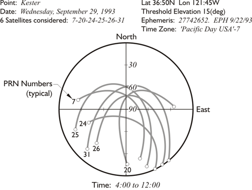
Polar Plot
One such diagram is a plot of the satellite’s tracks drawn on a graphical representation of the upper half of the celestial sphere with the observer’s zenith at the center and perimeter circle as the horizon. The azimuths and elevations of the satellites above the specified 15-degree mask angle are connected into arcs that represent the paths of all available satellites. The utility of this sort of drawing has lessened with the completion of the GPS/GNSS constellation. In fact, there are so many satellites available that the picture can become quite crowded and difficult to decipher.
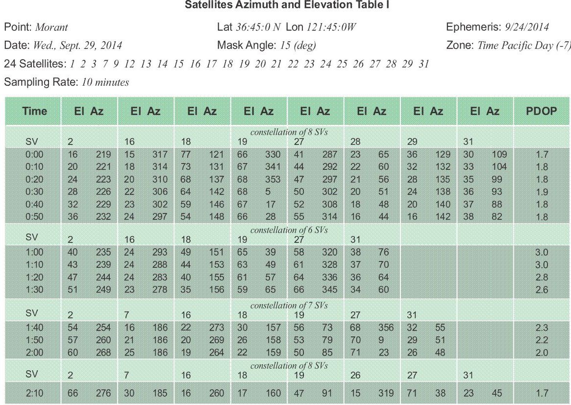
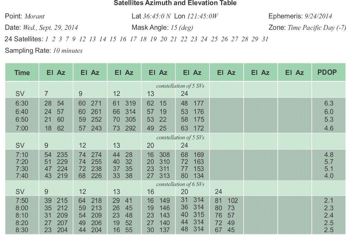
An example: the position of point Morant in the table needed expression to the nearest minute only, a sufficient approximation for the purpose. The ephemeris data were 5 days old when the chart was generated by the computer, but the data were still an adequate representation of the satellite’s movements to use in planning. The mask angle was specified at 15°, so the program would consider a satellite set when it moved below that elevation angle. The zone time was Pacific Daylight Time, 7 hours behind Coordinated Universal Time, UTC. The full constellation provided 24 healthy satellites, and the sampling rate indicated that the azimuth and elevation of those above the mask angle would be shown every 10 minutes. This is all in view. You could use this to plan particular observation windows when four or more satellites were up, the PDOP over there on the far right was at an acceptable level. These all seem to be fairly good. And then, one can plan the periods that you'll be observing from particular stations.
At 0:00 hour, satellite PRN 2 could be found on an azimuth of 219° and an elevation of 16° above the horizon by an observer at 36°45'Nf and 121°45'W?. The table indicates that PRN 2 was rising, and got continually higher in the sky for the 2 hours and 10 minutes covered by the chart. The satellite PRN 16 was also rising at 0:00, but reached its maximum altitude at about 1:10 and began to set. Unlike PRN 2, PRN 16 was not tabulated in the same row throughout the chart. It was supplanted when PRN 7 rose above the mask angle and PRN 16 shifted one column to the right. The same may be said of PRN 18 and PRN 19. Both of these satellites began high in the sky, unlike PRN 28 and PRN 29. They were just above 15° and setting when the table began and set after approximately 1 hour of availability. They would not have been seen again at this location for about 12 hours. This chart indicated changes in the available constellation from eight space vehicles, SVs, between 0:00 and 0:50, six between 1:00 and 1:30, seven from 1:40 to 2:00 and back to eight at 2:10. The constellation never dipped below the minimum of four satellites, and the PDOP was good throughout. The PDOP varied between a low of 1.7 and a high of 3.0. Over the interval covered by the table, the PDOP never reached the unsatisfactory level of 5 or 6, which is when a planner should avoid observation.
Choosing the Window
Using this chart, the GPS/GNSS survey designer might well have concluded that the best available window was the first. There was nearly an hour of 8-satellite data with a PDOP below 2. However, the data indicated that good observations could be made at any time covered here, except for one thing: it was the middle of the night.
Ionospheric Delay
It is worth noting that the ionospheric error is usually smaller after sundown. In fact, the FGDC specified dual-frequency receivers for daylight observations for the achievement of the highest accuracies, due, in part, to the increased ionospheric delay during those hours. When planning the survey, it's always useful to note that the ionospheric error is smaller after sundown. The table above shows data from later in the day. It covers a period of two hours when a constellation of 5 and 6 satellites was always available. However, through the first hour, from 6:30 to 7:30, the PDOP hovered around 5 and 6. For the first half of that hour, four of the satellites—PRN 9, PRN 12, PRN 13, and PRN 24—were all near the same elevation. During the same period, PRN 9 and PRN 12 were only approximately 50° apart in azimuth, as well. Even though a sufficient constellation of satellites was constantly available, the survey designer may well have considered only the last 30 to 50 minutes of the time covered by this chart as suitable for observation. There is one caution, however. Azimuth-elevation tables are a convenient tool in the division of the observing day into sessions, but it should not be taken for granted that every satellite listed is healthy and in service. For the actual availability of satellites and an update on atmospheric conditions, it is always wise to check. In the planning stage, the diligence can prevent creation of a design dependent on satellites that prove unavailable. Similarly, after the field work is completed, it can prevent inclusion of unhealthy data in the postprocessing.
Supposing that the period from 7:40 to 8:30 was found to be a good window, the planner may have regarded it as a single 50-minute session, or divided it into shorter sessions. One aspect of that decision was probably the length of the baseline in question. In static GPS/GNSS, a long line of 30 km may require 50 minutes of 6-satellite data, but a short line of 3 km may not. Another consideration was probably the approximation of the time necessary to move from one station to another.